Physical Parameters
Preface
My first concern with the physical parameters of the bicycle and rider occurred in my multi-body dynamics class project [Moo06]. There I developed a method of estimating the parameter values using simply the geometry and mass of the bicycle and rider. It was eventually presented as part of a paper at the 2008 ISEA conference in Biarritz, France [MH08]. This method served me well until more accurate estimates of the parameters were needed for the first instrumented bicycle I helped build at TU Delft, see Chapter Delft Instrumented Bicycle. I signed on to the task of measuring the bike’s physical parameters using the equipment and procedures developed in [Koo06] and to combine the results with my basic human model from [MH08] for the estimation of the complete system parameters of the Whipple model. These first measurements and the details of the human model were eventually presented in [MKHS09]. During this work, Dr. Hubbard encouraged me to think about the accuracy of the measurements in more detail, as some of the practices we were using were not as accurate as they could be. With that in mind and the fact that there was very little complete data available on the physical parameters of real bicycles, I decided to measure an assortment of bicycles we had available around the lab in Delft [MHP+10]. From this tedious task a rich data set was created and the measurement methodology tightened up considerably. Once I was back in Davis, we setup almost identical equipment to measure the two new bicycles we were constructing, see Chatper Davis Instrumented Bicycle. Danique Fintelman helped us come up with a more accurate geometry measurement. Steven Yen also used the equipment to measure a children’s bicycle with a gyro wheel. With one last improvement, we updated the human parameter estimates when Chris Dembia implemented Yeadon’s human inertia model and it was combined with the accurate bicycle measurements. These final methods for both bicycle and rider are implemented in two open source software packages.
Bicycle Parameters
Accurate measurements of a bicycle’s physical parameters are required for realistic dynamic simulation and analysis. The most basic models require the geometry, mass, mass location, and mass distributions for the rigid bodies. More complex models require estimates of tire characteristics, human body segment inertial characteristics, friction, stiffness, damping, etc. In this chapter I present the measurement of the minimal bicycle/rider parameters required for the benchmark Whipple bicycle model presented in [MPRS07]. This model is composed of four rigid bodies, has ideal rolling and frictionless joints, and is laterally symmetric. A set of 25 parameters describes the geometry, mass, mass location and mass distribution of each of the rigid bodies. The experimental methods used to estimate the parameters described herein are based primarily on the work done in [Koo06], [KSM08] and [MKHS09] but have been refined for improved accuracy and methodology.
Koojiman’s work was preceded by that of several others. Roland and Massing [RM71] measured the physical parameters of a bicycle in much the same way as is presented, including calculations of uncertainty from the indirect measurement techniques. [VZ75] measured the inertial parameters of his robotic bicycle with a swing pendulum and a stop watch. Patterson [Pat04b] used a swing to measure the roll inertia of recumbent bicycles with a rider. [Con09] and [Ste09] used a computer aided design package to estimate the parameters. [ER10] measured a bicycle for his bicycle dynamics class in Spain. Also, some notable motorcycle and scooter measurements include [Doh53], [Doh55], [SG71], [Eat73b], [RR73], and [Sha97].
Here is documented the indirect measurement of ten real bicycles’ physical parameters. We improve upon previous methods by both increasing and reporting the accuracies of the measurements and by measuring the complete moments of inertia of the laterally symmetric frame and fork needed for analysis of the nonlinear model. Furthermore, very little data exists on the physical parameters of different types of bicycles and this work aims to provide a small sample of bicycles.
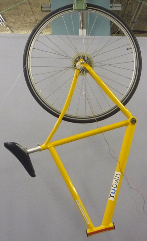
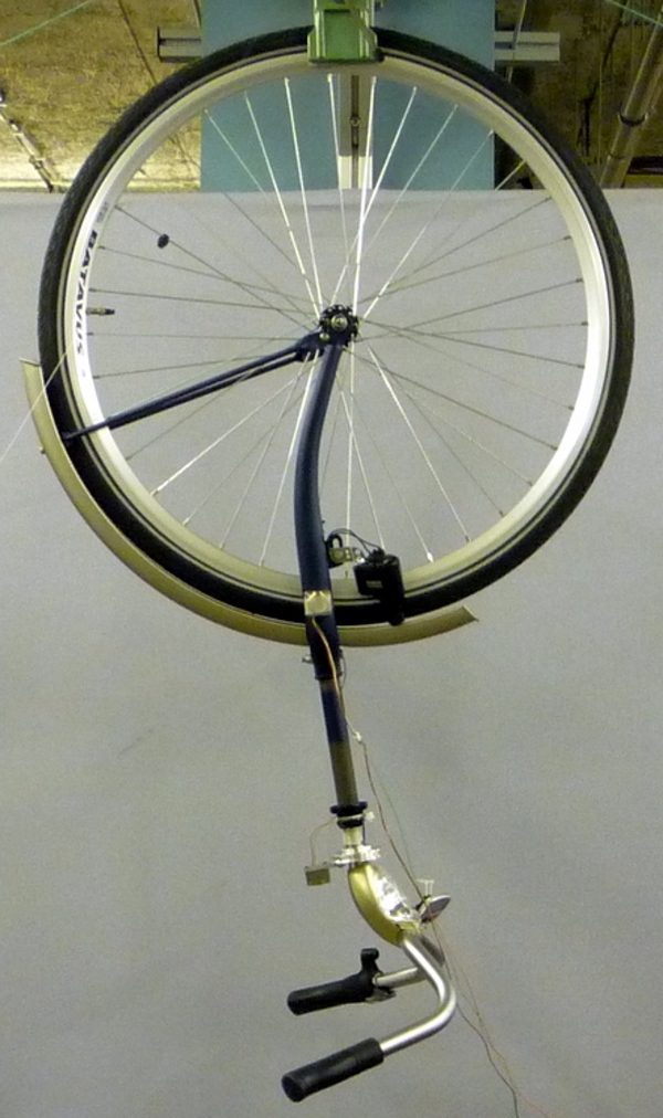
We measured the physical characteristics of eleven different bicycles, three of which were set up in two different configurations. The first six bicycles, chosen for both variety and convenience, are as follows: Batavus Browser, a Dutch style city bicycle measured with and without instrumentation as described in [KSM09]; Batavus Stratos Deluxe, a Dutch style sporty city bicycle; Batavus Crescendo Deluxe a Dutch style city bicycle with a suspended fork; Gary Fisher Mountain Bike, a hard-tail mountain bicycle; Bianchi Pista, a modern steel frame track racing bicycle; and Yellow Bicycle, a stripped down aluminum frame road bicycle measured in two configurations, the second with the fork rotated in the head tube 180 degrees for larger trail. The last two bicycles were measured in Davis: the instrumented bicycle presented in chapter Davis Instrumented Bicycle and a children’s bicycle with a stabilizing flywheel called the GyroBike.
These eleven different parameter sets can be used with, but are not limited to, the benchmark bicycle model. The accuracy of all the measurements are presented. The accuracies are based measurement inaccuracies and the proper use of error propagation theory with correlations taken into account.
Parameters
Of primarily concern was measuring and estimating the 25 parameters associated with the benchmark Whipple bicycle model which is derived and described in [MPRS07]. The unforced two degree-of-freedom, \(\mathbf{q} = [\delta \quad \phi]^T\) model takes the form:
where the entries of the \(\mathbf{M}\), \(\mathbf{C}_1\), \(\mathbf{K}_0\) and \(\mathbf{K}_2\) matrices are combinations of 25 bicycle physical parameters that include the geometry, mass, mass location and mass distribution of the four rigid bodies. The 25 parameters presented in [MPRS07] are not necessarily a minimum set for the Whipple model, as shown in [Sha08], but are useful none-the-less as they represent intuitively measurable quantities and have become become standard due to the nature of the benchmark. They are also not parameters used in directly in the derivation in Chapter Bicycle Equations Of Motion but can easily be converted, as was shown. The 25 parameters can be measured using many techniques. In general, I attempted to measure the benchmark parameter as directly as possible to improve the accuracy.
Bicycle Descriptions
We measured a total of eight bicycles in eleven configurations, Figure 5.1. The three Batavus bicycles were donated by the manufacturer. We asked for a bicycle that they considered stable and one that they did not. They offered the Browser as a “stable” bicycle and the Stratos as “nervous”. The Crescendo was considered average handling. We measured an instrumented version of the Browser that was used in the experiments described in Chapter Delft Instrumented Bicycle. The Fisher and the Pista were chosen to provide some variety, a mountain and road bike. The yellow bike is used to demonstrate bicycle stability and the forked is reversed to provide better stability when perturbed with no rider. The Davis instrumented bicycle is an instrumented bicycle described in Chapter Davis Instrumented Bicycle and we measured the frame in configurations for different rider seating positions. The child’s bicycle has the GyroWheel product installed in the front wheel. The first six of these bicycles were measured in Delft and will hereafter be referred to as the Delft Bicycles. The remaining two bicycles were measure in Davis and will be referred to as the Davis Bicycles.
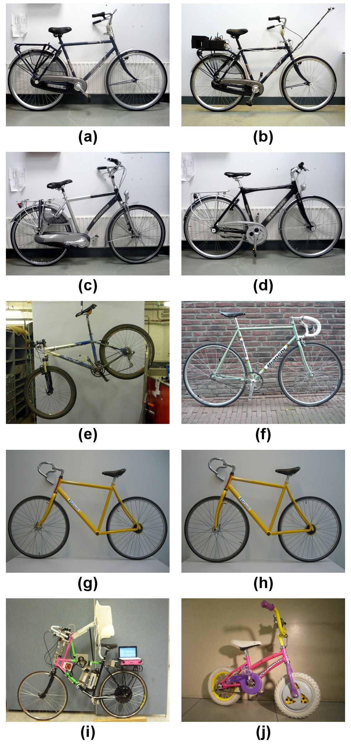
The ten measured bicycles: (a) Batavus Browser, (b) Instrumented Batavus Browser, (c) Batavus Crescendo Deluxe, (d) Batavus Stratos Deluxe, (e) Gary Fisher, (f) Bianchi Pista, (g) Yellow Bicycle, (h) Yellow Bicycle with reversed fork, (i) Davis Instrumented Bicycle, (j) Gyro Bicycle. The Davis Instrumented Bicycle was measured twice each with the body cast and seat height in different positions. The first “Rigid” was set up for Jason and the second “Rigidcl” was set up for Luke and Charlie. Only one image of the Rigid bicycle is shown, even though it was measured in two slightly different configurations.
Accuracy
We here analyze the accuracy of the measurements of the parameters. Following the lead of [RM71] error propagation theory was used to calculate accuracy of the 25 benchmark parameters. This begins by estimating the standard deviation of the actual measurements taken, see Section Bicycle Measured Parameters. The measurement error was chosen based on the measuring tool and methods used. If \(x\) is a parameter and is a function of the measurements, \(u,v,\ldots\), which are Gaussian random variables then \(x\) is also a Gaussian random variable defined as \(x=f(u,v,\ldots)\). The sample variance of \(x\) is defined as
Using the definitions for variance and covariance, Equation (2) can be simplified to
If \(u\) and \(v\) are uncorrelated then \(s_{uv}=0\). Most of the calculations hereafter have uncorrelated variables but a few do not and the covariance has to be taken into account. Equation (3) can be used to calculate the variance of all types of functions. I made use of the Python package uncertainties [Leb10] to simplify the book keeping of the correlations and variance calculations, thus some of the equations for the error are not shown in the following sections.
Geometry
The geometry measurements of the Delft bicycles focused on measuring the benchmark parameters: trail, wheelbase, and steer axis tilt as directly as possible. I also present an alternative method for the geometry used with the Davis bicycles that attempts to measure the distances in my model derivation, Chapter Bicycle Equations Of Motion, which improves the accuracy of the parameters. Keep in mind, that I assumed that the frame did not flex and that the wheel radii do not change with rider weight when taking geometric measurements.
Wheel Radii
The radii of the front \(r_\mathrm{F}\) and rear \(r_\mathrm{R}\) wheels were estimated by measuring the linear distance traversed along the ground through at least ten rotations of the wheel. Each wheel traversal was measured separately and the measurements were taken with rider seated on the bicycle, except for the gyro bicycle which had no rider. A 72 kg rider sat on the Delft bicycles and an 84 kg rider on the Davis instrumented bicycle [1]. A 30 meter tape measure (resolution: 2mm) was pulled tight and taped on a flat level smooth floor for the Delft bicycles and for the Davis bicycles we marked a 68 foot length on the floor and used a 1/16 inch resolution ruler to measure the 6 to 15 inch distance past the 68 foot mark where the rotation stopped. The tire was marked and aligned with the tape measure Figure 5.2. The accuracy of the distance measurement is approximately \(\pm0.01\) meter. The tires were pumped to the recommended inflation pressure before the measurements. The wheel radius is calculated by
where \(r\) is the wheel radius, \(d\), is the traversal distance, \(n\), is the number of rotations and \(\sigma\) is the respective standard deviation of the subscripted variable. I use subscripts \(F\) and \(R\) from front and rear wheels, respectively, in the measurement tables in Section Bicycle Measured Parameters.
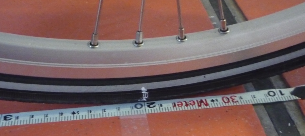
Wheel and tire with chalk mark aligned to the tape measure.
Head Tube Angle
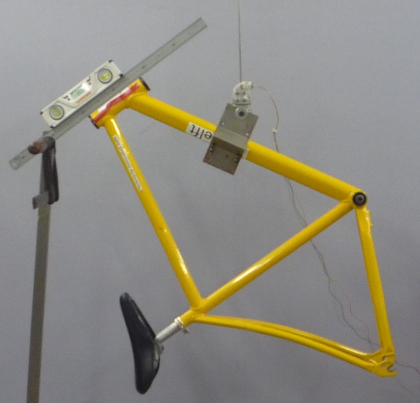
For the Delft Bicycles, the head tube angle was measured directly using an electronic level, Figure 5.3. The bicycle frame was fixed perpendicular to the ground, the steering angle was set to the nominal position, tire pressures were at recommended levels, and the bicycle was unloaded. The steer axis tilt \(\lambda\) is the complement to the head tube angle, \(\gamma\).
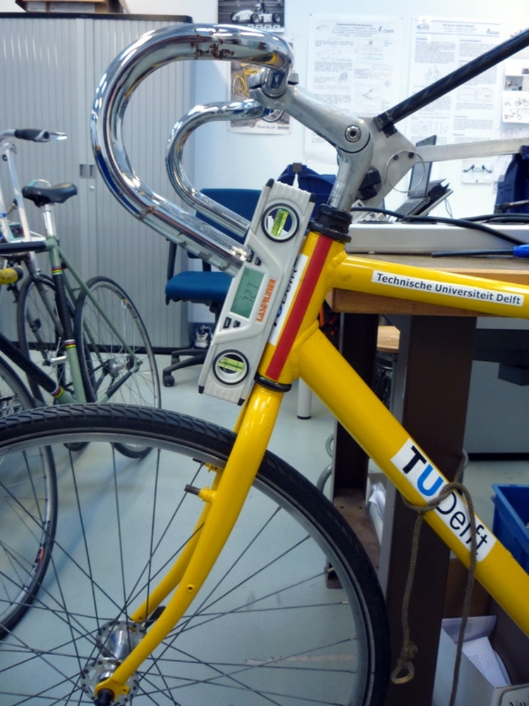
The digital level set against the Yellow Bicycle’s head tube.
Trail
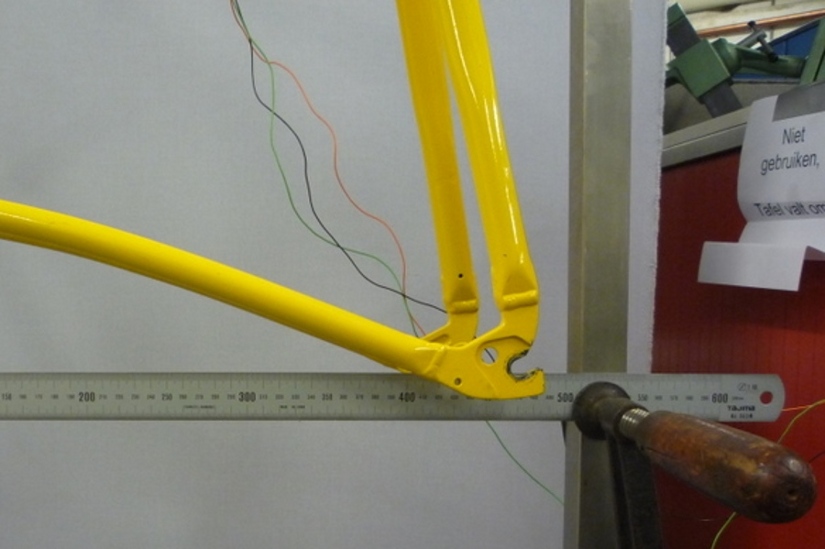
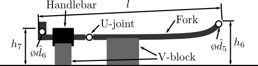
The idealized trail is difficult to measure directly due to the fact that the tire has a contact patch and there is no distinct contact point. Instead I chose to measure the fork offset, \(f_o\), and compute the ideal trail. The fork offset was measured by clamping the steer tube of the front fork into a v-block on a flat table, Figure 5.4. For the Delft bicycles, a ruler was used to measure the height of the center of the head tube and the height of the center of the axle axis, and for the Davis bicycles we made use of more accurate height gages. The fork blades were aligned such that the axle axis was parallel to the table surface.

The fork of the Davis Bicycle setup for measuring the fork offset.
Wheelbase
I measured the wheelbase directly with the bicycle in nominal configuration described in Section Head Tube Angle. We used a tape measure to measure the distance from one wheel axle center to the other.
Alternative Geometry Measurement Method
The geometry for the bicycle model presented in Chapter:eom can almost be measured directly. I used this method for the Davis Bicycles. The bicycle frame is set on a granite measurement table such that the head tube is in a v-block and parallel to the table surface and the bicycle frame is situated such that the frame is perpendicular to the table surface, Figure 5. The fork is rotated in the head tube such that the fork blades curve upwards. Two dummy axles are fit into the front and rear dropouts and the axles are ensured to be parallel to the table surface. The height from the table surface to the top of each axle are recorded with a height gage and the diameters of the axles are measured with a micrometer or caliper.
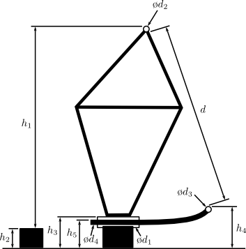
The actual measurements taken to compute the basic bicycle geometry.
These measurements can then be converted to the three essential bicycle dimensions, \(d_1\), \(d_2\), \(d_3\) described in Chapter Bicycle Equations Of Motion.
The traditional [MPRS07] parameters can then be calculated. If \(r_F\) does not equal \(r_R\) then the steer axis tilt cannot be computed analytically as Equation (11) holds.
It is trivial to find the solution to Equation (11) numerically. If \(r_F=r_R\), the solution for \(\lambda\) is analytic.
The wheelbase is
and trail is then computed with Equation (6), realizing \(f_o = d_3\):
Mass
For the Delft bicycles, each of the four bicycle parts were measured using a Molen 20 kilogram scale with a resolution of 20 grams, Figure 5.6. The accuracy was conservatively assumed to also be \(\pm20\) grams. Also, the total mass was measured using a spring scale with a resolution of 100 grams. The total mass was only used for comparison purposes, as it was not very accurate. The masses of the parts of the Davis bicycles were measured with a digital scale with a resolution of 50 grams (A & D FV-150k Industrial Scale).
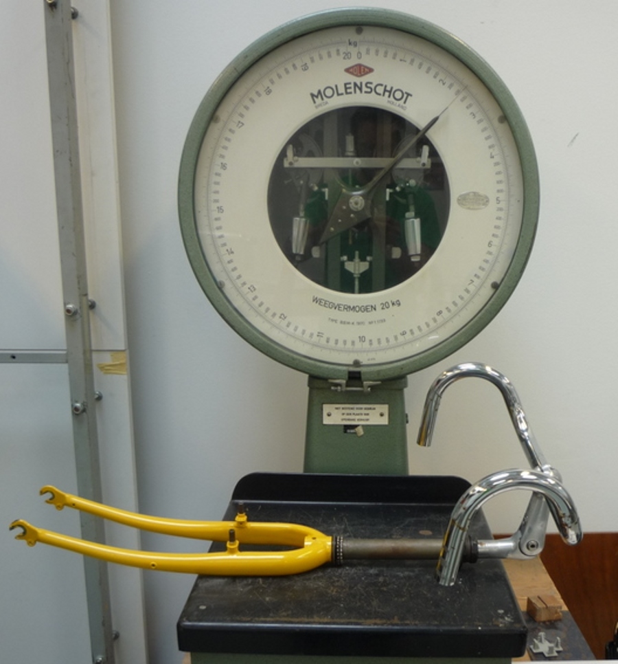
The scale used to measure the mass of each Delft bicycles’ components.
Center of Mass
Wheels
The centers of mass of the wheels were assumed to be at their geometrical centers to comply with the Whipple model. This was also assumed for the flywheel in the gyro bike.
Rear Frame
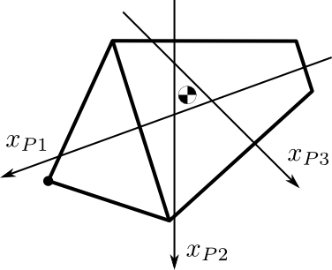
The rear frame bicycle configuration was hung in at least three orientations through the assumed lateral plane of symmetry. I assumed that the frame was laterally symmetric, complying with the Whipple model, thus reducing the need to use a more complex three dimensional measurement setup. The frame could rotate about a joint such that gravity aligned the center of mass with the support rod axis. The orientation angle of the steer axis, \(\alpha_\mathrm{B}\), see Figure 5.7, relative to the earth was measured using a digital level (\(\pm0.2^{\circ}\) accuracy), Figure 5.8. A thin string was aligned with the pendulum axis which passed by the frame. The horizontal distance \(a_\mathrm{B}\) between the rear axle and the string was measured by aligning a 1 mm resolution ruler perpendicular to the string Figure 5.9. The distance \(a_\mathrm{B}\) was negative if the string fell to the right of the rear axle and positive if it fell to the left of the rear axle, when viewing the bicycle from the right side. These measurements allow for the calculation of the center of mass location in the global reference frame.
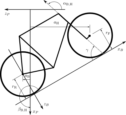
Pictorial description of the angles and dimensions that related the nominal bicycle reference frame \(XYZ_B\) with the pendulum reference frame \(XYZ_P\).
The digital level was mounted to a straight edge aligned with the head tube of the bicycle frame. This was done without allowing the straight edge to touch the frame. The frame was not absolutely stationary so this was difficult. The light frame oscillations could be damped out by submerging a low hanging area of the frame into a bucket of water to decrease the oscillation.
Measuring the distance from the pendulum axis to the rear wheel axle using a level ruler.
The frame rotation angle \(\beta_\mathrm{B}\) is defined as rotation of the frame in the nominal benchmark configuration to the hanging orientation, rotated about the \(Y\) axis.
The center of mass can be found by realizing that the pendulum axis \(X_P\) is simply a line in the nominal bicycle reference frame with a slope \(m\) and a z-intercept \(b\) where the \(i\) subscript corresponds to the different frame orientations, see Figure 5.10. The slope can be shown to be
Exaggerated intersection of the three pendulum axes and the location of the center of mass.
The z-intercept can be shown to be
Theoretically, the center of mass lies on each line but due to experimental error, if there are more than two lines, the lines do not all cross at the same point. Only two lines are required to calculate the center of mass of the laterally symmetric frame, but more orientations increase the center of mass measurement accuracy. The three lines are defined as
The mass center location can be calculated by finding the intersection of pairs of these three lines. Two approaches were used used to calculate the center of mass. Intuition leads one to think that the center of mass may be the centroid of the triangle made by the three intersecting lines. The centroid can be found by calculating the intersection point of each pair of lines and then averaging the three intersection points[2].
Fork and Handlebar
The fork and handlebars are generally a bit trickier to hang in three different orientations, Figure 5.11. Typically two angles can be obtained by clamping to the steer tube at the top and the bottom. The third angle can be obtained by clamping to the stem. The center of mass of the fork is calculated in the same fashion as the frame. The slope of the line in the benchmark reference frame is the same as for the rear frame but the z-intercept is different
The Stratos fork and handlebar assembly hung as a torsional pendulum.
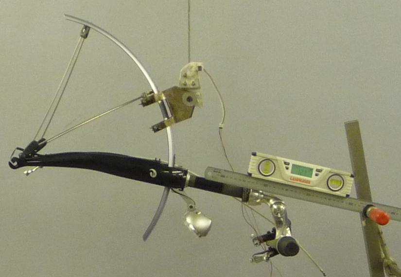
The fork of the Davis instrumented bicycle was connected to the handlebars by a steer torque sensor with universal joint. Due to the fact that the sensor and joint were not designed to support the weight of the adjacent components and the fact that we needed the inertia of the portion above the torque sensor for proper estimation of the steer torque applied by the rider[3], we opted to measure the center of mass and inertia of the fork and handlebar separately. The fork was measured as previously described, with the universal joint locked in its nominal position. The handlebar was measured in a similar fashion making use of small clamps to hang it in different orientations, Figure 5.12.
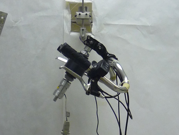
The handlebar mounted as a torsional pendulum.
I choose the center of the stem clamp bolt to be the reference point (as were the front and rear wheel centers for the front and rear frames). The location of this point relative to the front wheel center was measured as shown in Figure 5.13.
A diagram of how the handlebar reference point was located with respect to the front wheel center. These were the raw measurements taken.
The distances along and perpendicular to the steer axis from the front wheel center to the handlebar reference point are as follows
The distance from the front wheel center to the handlebar reference point in the global bicycle reference frame are
The center of mass is computed with respect to the handlebar reference point and \(u_1\) and u_2 locate the reference point of the handlebar to the front wheel center and thus the global origin.
Inertia
The moments of inertia of the wheels, rear frame, and fork (and handlebar) were measured both by taking advantage of the assumed symmetry of the parts and by hanging the parts as both compound and torsional pendulums while measuring their periods of oscillation when perturbed at small angles. The rate of oscillation was measured using a Silicon Sensing CRS03 100 deg/s rate gyro for the Delft bicycles and a Silicon Sensing CRS04 200 deg/s rate gyro for the Davis bicycles. The rate gyros were sampled at 1000 hz with a National Instruments USB-6008 12 bit data acquisition unit and at 500 hz with a National Instruments USB-6218 16 bit data acquisition unit, respectively, and the Matlab data acquisition toolbox. The measurement durations were between 15 and 30 secs and each moment of inertia measurement was performed at least three times. No extra care was taken to calibrate the rate gyro, maintain a constant power source (i.e. the battery drains slowly), or account for drift because I was only concerned with the period. The raw voltage signal was used to determine the period of oscillation which is needed for the moment of inertia calculations, Figure 5.14.

Example portion of the raw voltage data taken during a 30 second measurement of the oscillation of the Browser rear frame as a compound pendulum.
The function Equation (25) was fit to the data using the least squares method for each experiment to determine the quantities \(A\), \(B\), \(C\), \(\zeta\), and \(\omega\).
Most of the data fit the damped oscillation function well with very light (and potentially ignorable) damping. There were several instances in the Delft experiments of beating-like phenomena for some of the parts at particular orientations. Roland and Massing, [RM71], also encountered this problem and used a bearing to prevent the torsional pendulum from swinging. Figure 5.15 shows an example of the beating like phenomena. I used Roland and Massing’s solution to prevent this in the Davis measurements.

An example of the beating-like phenomena observed during less than 5% of the Delft trials.
The physical phenomenon observed corresponding to data sets such as these occurred when the bicycle frame or fork was perturbed torsionally. After being set into motion, the torsional motion damped and a longitudinal swinging motion increased. The motions alternated back and forth with neither ever reaching zero. The frequencies of these motions were very close to one another and it was not apparent how to dissect the two. We explored fitting to a function such as
But the fit predicts that \(\omega_1\) and \(\omega_2\) are very similar frequencies. There was no easy way to choose which of the two \(\omega\)‘s was the one associated with the torsional oscillation. Some work was done to model the torsional pendulum as a laterally flexible beam to determine this, but we ended up assuming that the accuracy of the period calculation would not improve enough for the effort required. The later experiments simply prevented the swinging motion of the pendulum without damping the torsional motion.
The period for a damped oscillation is
The uncertainty in the period, \(T\), can be determined from the fit. First, the variance of the fit is calculated
The covariance matrix of the fit function can be formed
where \(\mathbf{H}\) is the Hessian [Hubbard1989b] of the fit function, (25). \(\mathbf{U}\) is a \(5\times5\) matrix with the variances of each of the five fit parameters along the diagonal. The variance of \(T\) can be computed using the variance of \(\zeta\) and \(\omega\). It is important to note that the uncertainties in the period are very low (\(<1e-4\)) due to the high sample rate, even for the fits with low \(r^2\) values.
Torsional Pendulum
A torsional pendulum was used to measure all moments of inertia about axes in the laterally symmetric plane of each of the wheels, fork and frame. The pendulum is made up of a rigid mount, an upper clamp, a torsion rod, and various lower clamps, Figure 5.16 .
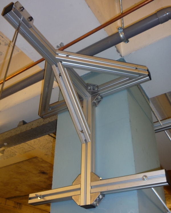
The rigid pendulum fixture from the Delft experiments mounted to a concrete column.
A mild steel rod was used as the torsion spring. Lightweight, relatively low moment of inertia clamps were constructed that could fix the torsional rod to the various bicycle parts. The moments of inertia of the clamps were neglected [4].
The torsional pendulum was calibrated using a rod with an easily computed, i.e. “known”, moment of inertia Figure 5.17[5]. A torsional pendulum almost identical to the one used in [Koo06] was used to measure the average period \(\overline{T}_i\) of oscillation of the rear frame at three different orientation angles \(\beta_i\), where \(i=1\), \(2\), \(3\), as shown in Figure 5.10. The parts were perturbed slightly, around 1 degree, and allowed to oscillate about the pendulum axis through several periods. This was repeated at least three times for each frame and the recorded periods were averaged.
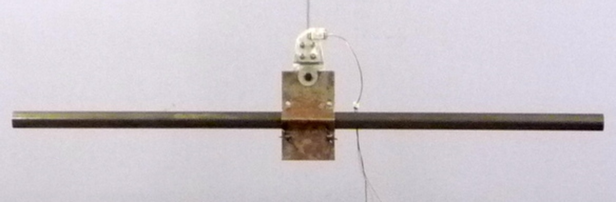
The steel calibration rod. The moment of inertia of the rod, \(I_P = \frac{m_P}{12}(3 r_P^2 + l_P^2)\), can be used to estimate the stiffness of the torsional pendulum, \(k = \frac{4 I_P \pi^2}{\overline{T_P}^2}\).
Wheels
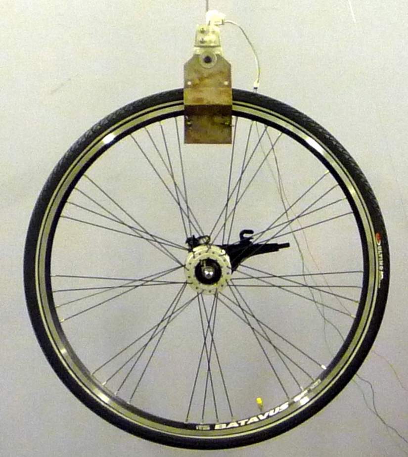
Estimating the full inertia tensors of the wheels is less complex because the wheels are assumed symmetric about three orthogonal planes making all products of inertia zero. The \(I_{xx}=I_{zz}\) moments of inertia were calculated by measuring the averaged period of oscillation about an axis in the \(XZ_B\)-plane using the torsional pendulum setup and Equation (32). The wheels are also assumed to be laterally symmetric about any radial axis. Thus only two moments of inertia are required for the set of benchmark parameters [MPRS07]. The moment of inertia about the axle was measured by hanging the wheel as a compound pendulum, Figure 5.18. The wheel was hung on a horizontal rod and perturbed to oscillate about the axis of the rod. The rate gyro was attached to the spokes near the hub[6] and oriented mostly along the axle axis. The wheels for the Delft bicycles would rotate at the rod contact point about the vertical axis which added a very low frequency component of rate along the vertical radial axis, but this should have little effect on the period estimation about the compound pendulum axis. A fixture was designed for the Davis bicycles that prevented undesired rotation. The pendulum length is the distance from the rod/rim contact point to the mass center of the wheel[7]. The inner diameter of the rim was measured and divided by two to get \(l_\mathrm{F,R}\). The moment of inertia about the axle is calculated from
A wheel hung as a compound pendulum.
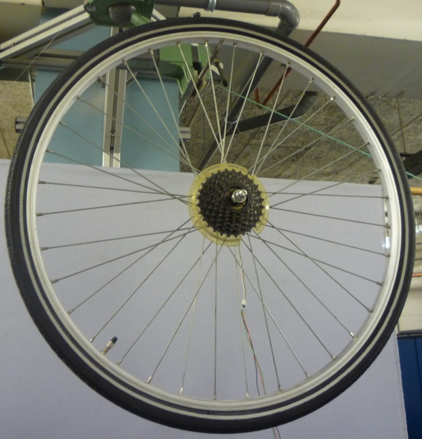
The radial moment of inertia was measured by hanging the wheel as a torsional pendulum, Figure 5.19. The wheel was first hung freely such that the center of mass aligned with the torsional pendulum axis and then the clamp secured. The wheel was then perturbed and oscillated about the vertical pendulum axis. The radial moment of inertia can be calculated with
The front wheel of the Crescendo hung as a torsional pendulum.
Frame
At least three measurements were made to estimate the locally level moments and products of inertia (\(I_{\mathrm{B}xx}\), \(I_{\mathrm{B}xz}\), and \(I_{\mathrm{B}zz}\)) of the rear frame in the nominal configuration. The rear frame was typically hung from either the three main tubes (seat tube, down tube, and top tube), the seat post, or a small fixture mounted to the brake mounts Figure 5.8. The rear fender prevented easy connection to the seat tube on some of the bikes and the clamp was attached to the fender. The fender was less rigid than the frame tube. For best accuracy with only three orientation angles, the frame should be hung at three angles that are \(120^\circ\) apart. Attaching by the three tubes on the frame generally provide that the orientation angles were spread evenly at about \(120^\circ\). Furthermore, taking data at more orientation angles improved the accuracy and was generally possible with standard diamond frame bicycles.
Three moments of inertia \(J_{\mathrm{B}i}\) about the pendulum axes were calculated using
The moments and products of inertia of the rear frame and handlebar/fork assembly with reference to the benchmark coordinate system were calculated by formulating the relationship between the rotated inertial frames
where \(\mathbf{J}_{\mathrm{B}i}\) is the inertia tensor about the pendulum reference frame, \(\mathbf{I}_\mathrm{B}\) is the inertia tensor in the locally level reference frame, and \(\mathbf{R}_{\mathrm{B}i}\) is the rotation matrix relating the two frames, Figure 5.7. The planar inertia tensor is defined as
The inertia tensor can be reduced to a \(2 \times 2\) matrix because the frame is assumed to be laterally symmetric and the \(Y\) axis of the pendulum reference is the same as the \(Y\) axis of the benchmark reference frame. The simple rotation matrix about the \(Y\)-axis can similarly be reduced to a \(2 \times 2\) matrix where \(s_{\beta i}\) and \(c_{\beta i}\) are defined as \(\sin{\beta_i}\) and \(\cos{\beta_i}\), respectively.
The first entry of \(\mathbf{J}_{\mathrm{B}i}\) in Equation (33) is the moment of inertia about the pendulum axis and is written explicitly as
Similarly, calculating all three, or more, \(J_{\mathrm{B}i}\) allows one to form
and the moments of inertia can be solved as a linear system or with least squares if it is over determined. The inertia of the frame about an axis normal to the plane of symmetry was estimated by hanging the frame as a compound pendulum about the wheel axis, Figure 5.20. Equation (30) is used but with the mass of the frame and the frame pendulum length.
The yellow bicycle rear frame hung as a compound pendulum about the wheel axis (the wheel is fixed in place).
Fork and handlebar
The inertia of the fork and handlebar is calculated in the same way as the frame. The fork is hung as both a torsional pendulum, Figure 5.11, and as a compound pendulum, Figure 5.21. The fork provides fewer mounting options to obtain at least three equally spaced orientation angles, especially if there is no fender. We designed a connection to the brake mounts for the Davis bicycles to remedy that. The torsional calculations follow equations (32) through (37) and the compound pendulum calculations is calculated with Equation (30). The fork pendulum length is calculated using
Browser fork hung as a compound pendulum.
Notation
The notation used in the bicycle parameter estimation.
- \(v\)
- Forward speed of the linear bicycle model.
- \(g\)
- Acceleration due to gravity.
- \(\mathbf{M},\mathbf{C}_1,\mathbf{K}_0,\mathbf{K}_2\)
- Velocity and gravity independent mass, damping, and stiffness matrices of the linearized Whipple model from [MPRS07].
- \(\mathbf{q}\)
- Essential coordinates from [MPRS07].
- \(\phi\)
- Roll angle.
- \(\delta\)
- Steer angle.
- \(\sigma\)
- Standard deviation. The subscript corresponds to the associated nominal variable.
- \(r_{(F,R)} \pm \sigma_{r(F,R)}\)
- Front \(F\) and rear wheel \(R\) radii and their respective standard deviations.
- \(d_{(F,R)} \pm \sigma_{d(F,R)}\)
- The traversed distance of each wheel.
- \(n_{(F,R)}\)
- The number of wheel rotations.
- \(\gamma \pm \sigma_\gamma\)
- The head tube angle and standard deviation.
- \(\lambda \pm \sigma_\lambda\)
- The steer axis tilt and standard deviation.
- \(f_o\)
- Fork offset.
- \(c \pm \sigma_c\)
- Trail and its standard deviation.
- \(d_1,d_2,d_3\)
- Fundamental bicycle geometry from Chapter Bicycle Equations Of Motion.
- \(d_1,d_2,d_3\)
- Fundamental bicycle geometry from Chapter Bicycle Equations Of Motion.
- \(d\)
- Inner dimension between the axles from the alternative geometry method.
- \(\hat{d}_1,\hat{d}_2,\hat{d}_3,\hat{d}_4\)
- Measured diameters from the alternative geometry method.
- \(h_1,h_2,h_3,h_4,h_5\)
- Measured heights from the table surface in the alternative geometry method.
- \(i\)
- Indices for each orientation of the front and rear frames in the pendulum.
- \(\alpha_{\mathrm{H,B}i}\)
- Angle of the steer axis relative to horizontal when the front frame and rear frame are hung as a pendulum.
- \(a_{\mathrm{H,B}i}\)
- Horizontal distance from the front or rear axle to the pendulum axis when the front and rear frames are hung as a pendulum.
- \(XYZ_P\)
- Pendulum reference frame.
- \(XYZ_{B}\)
- Global bicycle reference frame from [MPRS07].
- \(\beta_{\mathrm{H,B}i}\)
- Angle of the pendulum axis relative to the bicycle’s reference frame.
- \(m_{\mathrm{H,B}i}\)
- Slope of the pendulum axis in the bicycle reference frame.
- \(b_{\mathrm{H,B}i}\)
- Z intercept of the pendulum axis in the bicycle reference frame.
- \(z_{\mathrm{B}i}(x)\)
- Function describing the pendulum axis line in the \(XZ_B\) plane.
- \(\hat{d}_5,\hat{d}_6\)
- Handlebar and front wheel axle diameters.
- \(l\)
- The outer distance from the front wheel axle to the handlebar reference point.
- \(l_1,l_2\)
- The distances along and perpendicular to the steer axis from the front wheel center to the handlebar reference point.
- \(u_1,u_2\)
- The distances from the front wheel center to the handlebar reference point in the global bicycle reference frame.
- \(A,B,C\)
- The offset, sin amplitude, and cosine amplitude in the oscillations.
- \(\omega,\zeta\)
- The frequency and damping ratio in the oscillations.
- \(T\)
- Period of oscillation.
- \(\sigma_y\)
- The standard deviation of the measured voltage about the best fit curve.
- \(y_{mi}\)
- The measured voltage at each time.
- \(\bar{y}_m\)
- The mean of the measured voltage across all time.
- \(y_{pi}\)
- The predicted voltage value at each time.
- \(\mathbf{U}\)
- Covariance matrix of the fit function parameters.
- \(\mathbf{H}\)
- Hessian of the fit function parameters.
- \(\overline{T}_i\)
- Average period at orientation \(i\).
- \(I_P\)
- Inertia of the calibration rod about the pendulum axis.
- \(k\)
- Stiffness of the torsional pendulum.
- \(m_P\)
- Mass of the calibration rod.
- \(r_P\)
- Radius of the calibration rod.
- \(l_P\)
- Length of the calibration rod.
- \(T_P\)
- Oscillation period of the calibration rod.
- \(l_\mathrm{F,R}\)
- Front and rear wheel compound pendulum length.
- \(I_{Fyy},I_{Ryy}\)
- Moment of inertia of the front and rear wheels about the axle.
- \(I_{\mathrm{F,R}xx}\)
- Moment of inertia of the front and rear wheels about the radii.
- \(I_{\mathrm{B}xx},I_{\mathrm{B}xz},I_{\mathrm{B}zz}\)
- Moments and products of inertia of the rear fame with reference to the bicycle reference frame and the center of mass.
- \(\mathbf{I}_\mathrm{H,B}\)
- The inertia tensor of the front and rear frame with reference to the bicycle reference frame and the center of mass.
- \(\mathbf{J}_{\mathrm{H,B}i}\)
- The inertia tensor of the front and rear frame with reference to the pendulum reference frame and the center of mass for each orientation.
- \(\mathbf{R}_i\)
- The rotation matrix relating the pendulum and bicycle reference frames.
- \(s_{\beta i},c_{\beta i}\)
- Shorthand for \(\sin{\beta_i}\) and \(\cos{\beta_i}\).
- \(x_B,z_B\)
- The \(X\) and \(Z\) coordinates of the rear frame center of mass.
- \(l_B\)
- The rear frame pendulum length.
- \(x_H,z_H\)
- The \(X\) and \(Z\) coordinates of the front frame center of mass.
- \(l_H\)
- The front frame pendulum length.
Human Parameters
To properly model the bicycle rider system it is necessary to estimate the physical parameters of the bicycle rider. The measurement of the physical properties of a human is more difficult than for a bicycle because the human body parts are not as easily described as rigid bodes with defined joints and due to flexible geometry, daily varying mass, wobbly mass, etc.
Human mass, center of mass, and inertial properties have been measured and estimated in a multitude of ways. Each method has its advantages and disadvantages. Many methods exist including cadaver measurements ([Dem55], [CMY69], [CCM+75]), photogrammetry, ray scanning techniques ([ZS83], [ZSC90]), water displacement ([PKP99]), rotating platforms ([GWS05]), and geometrical estimation of the body segments ([Yea90a]). [Doh53], [Eat73b], and [Pat04b] measured the moments of inertia and centers of mass of a combined rider and vehicle, but this is not always practical especially if the properties of multiple riders are desired.
I approached the human parameter estimation in a more analytical fashion based primarily on geometric measurements much like Yeadon. Both methods that were used were based on estimating the inertial parameters from mass and geometry measurement along with a human body density estimate. With the first method, I estimated the physical properties of the rider in a seated position using a simple mathematical geometrical estimation similar in idea to [Yea90a] in combination with mass data from [Dem55]. The second method substitutes Yeadon’s more robust model with my previous one.
Simple Geometry Method
This method calculates the center of mass and inertia of a simplified model of the ten major human body parts: head, torso, upper and lower arms, and upper and lower legs, in a general configuration for sitting on typical bicycles. The mass of the rider was measured along with fourteen anthropometric measurements of the body. These measurements in combination with the geometrical bicycle measurements taken in the previous section (Bicycle Parameters) and several additional bicycle geometrical measurements are used to define a model of the rider made up of simple geometrical shapes (Figure 5.22). The legs and arms are represented by cylinders, the torso by a cuboid and the head by a sphere. The feet are positioned at the center of the bottom bracket axis to maintain symmetry about the \(XZ\)-plane.
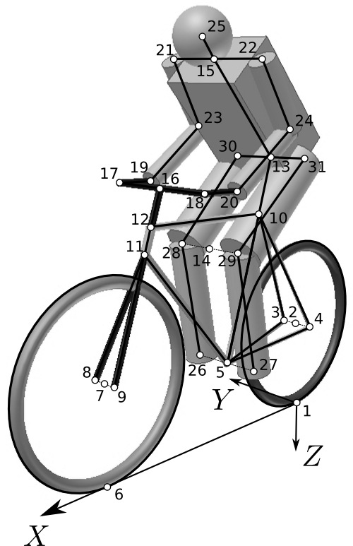
Locations of grid points and simple geometric shapes of the simple geometric inertia model.
All but one of the anthropomorphic measurements are taken when the rider was standing casually on flat ground. The lower leg length \(l_{ll}\) is the distance from the floor to the knee joint. The upper leg length \(l_{ul}\) is the distance from the knee joint to the hip joint. The length from hip to hip \(l_{hh}\) and shoulder to shoulder \(l_{ss}\) are the distances between the two hip joints and two shoulder joints, respectively. The torso length \(l_{to}\) is the distance between hip joints and shoulder joints. The upper arm length \(l_{ua}\) is the distance between the shoulder and elbow joints. The lower arm length \(l_{al}\) is the distance from the elbow joint to the center of the hand when the arm is outstretched. The circumferences are taken at the cross section of maximum circumference (e.g. around the bicep, around the brow, over the nipples for the chest). The final dimension is taken while the rider is seated on the bicycle in a normal riding position. The forward lean angle \(\lambda_{fl}\) is the approximate angle made between the floor (\(XY\)-plane) and the line connecting the center of the rider’s head and the top of the seat. This was estimated by taking a side profile photograph of the rider on the bicycle and scribing a line from the center of the head to the top of the seat. The measurements were made as accurately as possible with basic tools but no special attention is given further to the accuracy of the calculations due to the fact that modeling the human as basic geometric shapes already introduces an unknown error.
I measured twelve additional geometric values (only five of which are needed for this setup[8]) to assist in configuring the rider to the be seated on the bicycle, Figure 5.23.
- \(h_{bb}\), Bottom Bracket Height
- The distance from the ground to the bottom bracket when the bicycle is in the nominal configuration.
- \(l_{cs}\), Chain stay length
- Not the true chain stay length, but the distance from the center of the bottom bracket to the center of the rear wheel.
- \(l_{sp}\), Seat post length
- The distance from the intersection of a horizontal top tube and the seat tube to the top of the seat. Measured along the center line of the seat post.
- \(l_{st}\), Seat tube length
- The distance from the bottom bracket to the point at which a horizontal top tube would intersect the seat tube.
- \(\lambda_{st}\), Seat tube angle
- The acute angle between the ground and the seat tube.
- \(l_{f}\), fork length[8]
- The distance from the center of the front wheel to the intersection of the head tube and the down tube.
- \(w_{fh}\), front hub width[8]
- The distance between the front dropouts.
- \(w_{hb}\), handlebar width[8]
- The distance between the handlebar grips.
- \(l_{hb}\), handlebar length[8]
- The horizontal distance from the steer axis to the handlebar grips.
- \(\lambda_{ht}\), head tube angle[8]
- The angle between the ground and the head tube.
- \(w_{rh}\), rear hub width[8]
- The distance between the rear dropouts.
- \(l_{s}\), stem length[8]
- The distance from the intersection of the top tube and the head tube to the level of the handlebar grips.
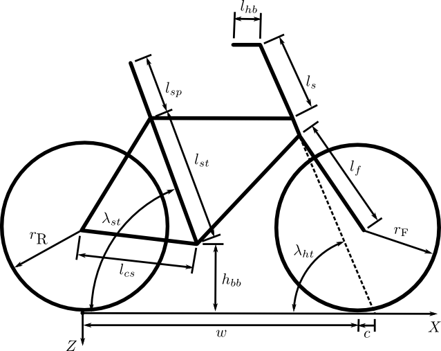
The dimensions need to construct the grid point system in the simple inertia method.
The masses of each segment (Table 5.1) were defined as a proportion of the total mass of the rider \(m_{\mathrm{B}r}\) using data from cadaver studies by [Dem55].
| Segment | Symbol | Equation |
| body | \(m_{B_r}\) | \(m_{B_r}\) |
| head | \(m_h\) | \(0.068 \cdot m_{B_r}\) |
| lower arm | \(m_{la}\) | \(0.022 \cdot m_{B_r}\) |
| lower leg | \(m_{ll}\) | \(0.061 \cdot m_{B_r}\) |
| torso | \(m_{to}\) | \(0.510 \cdot m_{B_r}\) |
| upper arm | \(m_{ua}\) | \(0.028 \cdot m_{B_r}\) |
| upper leg | \(m_{ul}\) | \(0.100 \cdot m_{B_r}\) |
The geometrical and anthropomorphic measurements are converted into a set of thirty one grid points in three dimensional space that map the skeleton of the rider and bicycle (Figure 5.22). The position vectors to these grid points are listed in Table 5.2. Several intermediate variables used in the grid point equations are listed in Table 5.3 where \(f_o\) is the fork offset and the rest arise due to multiple solutions to the location of the elbow and knee joints and have to be solved numerically. The correct solutions are the ones that force the arms and legs to bend in a natural fashion. The grid points mark the center of the sphere and the end points of the cylinders and cuboid. The segments are aligned along lines connecting the appropriate grid points.
| Description | Equation |
| rear contact point | \(\mathbf{r}_1=\left[0 \quad 0 \quad 0\right]\) |
| rear wheel center | \(\mathbf{r}_2=\left[0 \quad 0 \quad -r_\mathrm{R}\right]\) |
| right rear hub center | \(\mathbf{r}_3=\mathbf{r}_2+\left[0 \quad \frac{w_{rh}}{2} \quad 0\right]\) |
| left rear hub center | \(\mathbf{r}_4=\mathbf{r}_2+\left[0 \quad -\frac{w_{rh}}{2} \quad 0\right]\) |
| bottom bracket center | \(\mathbf{r}_5=\left[\sqrt{l_{cs}^2-(r_\mathrm{R}-h_{bb})^2} \quad 0 \quad -h_{bb}\right]\) |
| front wheel contact point | \(\mathbf{r}_6=\left[w \quad 0 \quad 0\right]\) |
| front wheel center | \(\mathbf{r}_7=\mathbf{r}_6+\left[0 \quad 0 \quad -r_\mathrm{F}\right]\) |
| right front hub center | \(\mathbf{r}_8=\mathbf{r}_7+\left[0 \quad \frac{w_{fh}}{2} \quad 0\right]\) |
| left front hub center | \(\mathbf{r}_9=\mathbf{r}_7+\left[0 \quad -\frac{w_{fh}}{2} \quad 0\right]\) |
| top of seat tube | \(\mathbf{r}_{10}=\mathbf{r}_5+\left[-l_{st}\cos{\lambda_{st}} \quad 0 \quad -l_{st}\sin{\lambda_{st}}\right]\) |
| fork crown | \(\mathbf{r}_{11}=\mathbf{r}_7+\left[-f_o\sin{\lambda_{ht}}-\cos{\lambda_{ht}}\sqrt{l_{f}^2-f_o^2} \quad 0 \quad f_o\cos{\lambda_{ht}}-\sin{\lambda_{ht}}\sqrt{l_{f}^2-f_o^2}\right]\) |
| top of head tube | \(\mathbf{r}_{12}=\left[r_{X11}-\frac{r_{Z11}-r_{Z10}}{\tan{\lambda_{ht}}} \quad 0 \quad r_{Z10}\right]\) |
| top of seat | \(\mathbf{r}_{13}=\mathbf{r}_{10}+\left[-l_{sp}\cos{\lambda_{st}} \quad 0 \quad -l_{sp}\sin{\lambda_{st}}\right]\) |
| center of knees | \(\mathbf{r}_{14}=\mathbf{r}_5+\left[s \quad 0 \quad -t\right]\) |
| shoulder midpoint | \(\mathbf{r}_{15}=\mathbf{r}_{13}+\left[l_{to}\cos{\lambda_{fl}} \quad 0 \quad -l_{to}\sin{\lambda_{fl}}\right]\) |
| top of stem | \(\mathbf{r}_{16}=\mathbf{r}_{12}+\left[-l_{s}\cos{\lambda_{ht}} \quad 0 \quad -l_{s}\sin{\lambda_{ht}}\right]\) |
| right handlebar | \(\mathbf{r}_{17}=\mathbf{r}_{16}+\left[0 \quad \frac{l_{ss}}{2} \quad 0\right]\) |
| left handlebar | \(\mathbf{r}_{18}=\mathbf{r}_{16}+\left[0 \quad -\frac{l_{ss}}{2} \quad 0\right]\) |
| right hand | \(\mathbf{r}_{19}=\mathbf{r}_{17}+\left[-l_{hb} \quad 0 \quad 0\right]\) |
| left hand | \(\mathbf{r}_{20}=\mathbf{r}_{18}+\left[-l_{hb} \quad 0 \quad 0\right]\) |
| right shoulder | \(\mathbf{r}_{21}=\mathbf{r}_{15}+\left[0 \quad \frac{l_{ss}}{2} \quad 0\right]\) |
| left shoulder | \(\mathbf{r}_{22}=\mathbf{r}_{15}+\left[0 \quad -\frac{l_{ss}}{2} \quad 0\right]\) |
| right elbow | \(\mathbf{r}_{23}=\mathbf{r}_{19}+\left[-u \quad \frac{l_{ss}}{2} \quad -v\right]\) |
| left elbow | \(\mathbf{r}_{24}=\mathbf{r}_{23}+\left[0 \quad -l_{ss} \quad 0\right]\) |
| center of head | \(\mathbf{r}_{25}=\mathbf{r}_{15}+\left[\frac{c_{h}}{2\pi}\cos{\lambda_{fl}} \quad 0 \quad -\frac{c_{h}}{2\pi}\sin{\lambda_{fl}}\right]\) |
| right foot | \(\mathbf{r}_{26}=\mathbf{r}_{5}+\left[0 \quad \frac{l_{hh}}{2} \quad 0\right]\) |
| left foot | \(\mathbf{r}_{27}=\mathbf{r}_{5}+\left[0 \quad -\frac{l_{hh}}{2} \quad 0\right]\) |
| right knee | \(\mathbf{r}_{28}=\mathbf{r}_{14}+\left[0 \quad \frac{l_{hh}}{2} \quad 0\right]\) |
| left knee | \(\mathbf{r}_{29}=\mathbf{r}_{14}+\left[0 \quad -\frac{l_{hh}}{2} \quad 0\right]\) |
| right hip | \(\mathbf{r}_{30}=\mathbf{r}_{13}+\left[0 \quad \frac{l_{hh}}{2} \quad 0\right]\) |
| left hip | \(\mathbf{r}_{31}=\mathbf{r}_{13}+\left[0 \quad -\frac{l_{hh}}{2} \quad 0\right]\) |
| Symbol | Equation |
| \(f_o\) | \(r_\mathrm{F}\cos{\lambda_{ht}}-c\sin{\lambda_{ht}}\) |
| \(s\) | \(0=l_{ul}^2-l_{ll}^2-(r_{Z13}-r_{Z5})^2-(r_{X5}-r_{X13})^2-2(r_{Z13}-r_{Z5})\sqrt{(l_{ll}^2-s^2)}-2s(r_{X5}-r_{X13})\) |
| \(t\) | \(\sqrt{l_{ll}^2-s^2}\) |
| \(u\) | \(0=l_{la}^2-l_{ua}^2+(r_{Z21}-r_{Z19})^2+(r_{X19}-r_{X21})^2+2(r_{Z21}-r_{Z19})\sqrt{(l_{la}^2-u^2)}-2u(r_{X19}-r_{X21})\) |
| \(v\) | \(\sqrt{l_{la}^2-u^2}\) |
The segments are assumed to have uniform density so the centers of mass are taken to be at the geometrical centers. The midpoint formula can then be used to calculate the local centers of mass for each segment in the global reference frame. The total body center of mass can be found from the standard formula
where \(\mathbf{r}_i\) is the position vector to the centroid of each segment and \(m_i\) is the mass of each segment. The local moments of inertia of each segment are determined using the ideal definitions of inertia for each segment type (Table 5.4).
| Segment | Inertia |
| cuboid | \(\frac{1}{12}m\begin{bmatrix}l_y^2+l_z^2 & 0 & 0\\0 & l_x^2+l_z^2 & 0\\0 & 0 & l_x^2+l_y^2\end{bmatrix}\) |
| cylinder | \(I_x\), \(I_y=\frac{1}{12}m\left(\frac{3c^2}{4\pi^2}+l^2\right)\), \(I_z=\frac{mc^2}{8\pi^2}\) |
| sphere | \(I_x\), \(I_y\), \(I_z=\frac{mc^2}{10\pi^2}\) |
The width of the cuboid representing the torso \(l_y\) is defined by the shoulder width and upper arm circumference.
The cuboid thickness was estimated using the chest circumference measurement assuming that the cross section of the chest is similar to a stadium shape.
The local \(\hat{\mathbf{z}}_i\) unit vector for the segments was defined along the line connecting the associated grid points from the lower numbered grid point to the higher numbered grid point. The local unit vector in the \(y\) direction was set equal to the global \(\hat{\mathbf{Y}}\) unit vector with the \(\hat{\mathbf{x}}_i\) unit vector following from the right hand rule. The rotation matrix needed to rotate each of the moments of inertia to the global reference frame can be calculated by dotting the global unit vectors \(\hat{\mathbf{X}}\), \(\hat{\mathbf{Y}}\), \(\hat{\mathbf{Z}}\) with the local unit vectors \(\hat{\mathbf{x}}_i\), \(\hat{\mathbf{y}}_i\), \(\hat{\mathbf{z}}_i\) for each segment.
The local inertia matrices are then rotated to the global reference frame with
The local moments of inertia can then be translated to the center of mass of the entire body using the parallel axis theorem
where \(d_x\), \(d_y\) and \(d_z\) are the distances along the \(X\), \(Y\) and \(Z\) axes, respectively, from the local center of mass to the global center of mass. Finally, the local translated and rotated moments of inertia are summed to give the total moment of inertia of the rider.
The results of measuring the riders are presented in Chapter Delft Instrumented Bicycle, Motion Capture, and [MKHS09].
Yeadon method
The [Yea90a] human inertial model was developed for estimating the inertial parameters needed to describe a human model for complex gymnastic maneuvers. It is essentially a more complete and accurate method than the one previously presented. There are 95 geometrical measurements of the human and a single mass measurement for scaling the body part densities. Yeadon makes use of stadium solids and a single semi-ellipse to more accurately model the human geometry. Two apparent deficiencies are the fact that too much detail is taken for body parts that have less inertia (i.e. the hands/feet) and at large configuration angles for some joints, the inertia is poorly modeled (e.g. the buttocks disappears when the human in a seated position). The model also does not have full freedom at each joint. Refer to [Yea90a] for a complete description of the model.
Once the inertia of each segment in the Yeadon model is computed, the joint angles must be set. We set the somersault angle to match the forward lean angle as described in the previous section. We then measure three additional bicycle dimensions to assist in the configuration of the rider. They are as follows:
- \(w_{hb}\), Handlebar width
- The lateral distance between the points the hands hold the handlebars.
- \(l_{hbR}\), Rear hub to handlebar.
- The distance from the center of the rear hub to the point on the handlebar where the hand grips.
- \(l_{hbF}\), Front hub to handlebar.
- The distance from the center of the front hub to the point on the handlebar where the hand grips.
We locate the hip center (Ls0) at the top of the bicycle seat and the somersault joint angle is set such that the torso (P, T, C) aligned by the forward lean angle \(\lambda_{fl}\).
The basic process for setting the elbow elevation angle is to find the distance between the shoulder (La0, Lb0) and the handlebar grip. The handlebar grip location is at the point at which the lateral line with length \(\frac{w_{hb}}{2}\) intersects the circle formed by the intersection of the two spheres which are centered at the front and rear wheel centers with radii \(l_{hbF}\) and \(l_{hbR}\), respectively. The elevation angle of the elbow then is defined as the angle at which the distance from the shoulder (La0, Lb0) to the knuckle (La6, Lb6) is equal to the distance from the shoulder (La0, Lb0) to the handlebar grip. We then assume that the shoulder rotation angle is zero and find the shoulder elevation and abduction angles which force the vector from the shoulder to the knuckle to equal the vector from the shoulder to the handlebar grip.
The thigh and knee elevation angles are set such that the center of the heel level (Lj6, Lk6) is aligned with the bottom bracket axis and that both the thigh abduction and rotation angles are zero. We assume that the foot peg is located at the bottom bracket center and is the same lateral distance from the sagittal plane as the hip centers. The knee and thigh elevation angles are then found in the same fashion as the elbow and shoulder angles, which the lesser restriction that the thigh abduction angle is zero.
Figure 5.24 shows a visualization of the Yeadon model when configured to sit on a bicycle. The details of the calculations and all of the data is included with the Yeadon [Dem11] and BicycleParameters [Moo11] software packages.
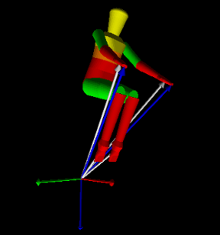
A visualization of the Yeadon inertia model configured to sit on a bicycle. Output is from the BicycleParameters software package.
Bicycle-Rider Parameters
Once both the bicycle and rider parameters are known, the parameter for various systems can be extracted. The simplest is that the rider is rigidly attached to the frame. The parallel axis theorem allows one to calculate the combined inertia of the bicycle frame and the rigid rider. Both of the rider formulations also allow one to segment the body for more complex rider models with multiple degrees of freedom. For example, the inertia for a leaning rider’s upper body can be determined separately and the legs can be fixed in the bicycle frame. We make use of this for the different rider biomechanical models presented in Chapter Extensions of the Whipple Model.
Software Implementation
The bicycle parameter calculation and the Yeadon method have been implemented in two open source software packages written in the Python language, called yeadon [Dem11] and BicycleParameters [Moo11]. The Yeadon package uses geometric measurements and joint configuration angles to output the total inertia properties of the human in an arbitrary reference frame. It also can provide inertial properties of individual body segments or combinations of body segments. It is suitable for a wide variety of human dynamic models. The BicycleParameters package accepts either the raw measurements described in Section Bicycle Parameters or the benchmark parameterization [MPRS07] and computes the benchmark bicycle parameters. It makes use of the Yeadon package to allow one to configure riders in a seated position on the bicycle and outputs the inertial properties of the bicycle/rider system. Overall it allows one to provide values and uncertainties for all of the raw measurements as described in both the Bicycle and Yeadon parameter sections and compute the parameters for the Whipple Bicycle model. Details of use of the software can be found in the documentation for each of the packages: http://packages.python.org/yeadon, http://packages.python.org/BicycleParameters.
Parameter Tables
The tabulated values for the both the raw measurements (Tables 5.5 to 5.8) and the computed physical parameters (Tables 5.9 to 5.12) of the ten bicycles are given in the following tables.
Bicycle Measured Parameters
| Browser | Browserins | Stratos | ||||
|---|---|---|---|---|---|---|
| Variable | \(v\) | \(\sigma\) | \(v\) | \(\sigma\) | \(v\) | \(\sigma\) |
| \(a_{B1}\) | 0.098 | 0.003 | -0.018 | 0.003 | 0.249 | 0.003 |
| \(a_{B2}\) | 0.169 | 0.003 | -0.355 | 0.003 | -0.267 | 0.003 |
| \(a_{B3}\) | -0.294 | 0.003 | -0.242 | 0.003 | -0.071 | 0.003 |
| \(a_{H1}\) | 0.474 | 0.003 | 0.474 | 0.003 | 0.329 | 0.003 |
| \(a_{H2}\) | 0.383 | 0.003 | 0.383 | 0.003 | -0.038 | 0.003 |
| \(a_{H3}\) | 0.215 | 0.003 | 0.215 | 0.003 | 0.400 | 0.003 |
| \(\alpha_{B1}\) | 3.4 | 0.2 | 154.1 | 0.2 | 128.9 | 0.2 |
| \(\alpha_{B2}\) | 138.7 | 0.2 | 230.8 | 0.2 | 221.6 | 0.2 |
| \(\alpha_{B3}\) | 229.8 | 0.2 | 286.9 | 0.2 | 184.5 | 0.2 |
| \(\alpha_{H1}\) | 346.7 | 0.2 | 346.7 | 0.2 | 36.0 | 0.2 |
| \(\alpha_{H2}\) | 28.1 | 0.2 | 28.1 | 0.2 | 94.0 | 0.2 |
| \(\alpha_{H3}\) | 287.0 | 0.2 | 287.0 | 0.2 | 347.3 | 0.2 |
| \(d_F\) | 28.06 | 0.01 | 27.98 | 0.01 | 27.77 | 0.01 |
| \(d_P\) | 0.0300 | 0.0001 | 0.0300 | 0.0001 | 0.0300 | 0.0001 |
| \(d_R\) | 27.85 | 0.01 | 27.84 | 0.01 | 29.77 | 0.01 |
| \(f\) | 0.070 | 0.001 | 0.070 | 0.001 | 0.045 | 0.001 |
| \(g\) | 9.81 | 0.01 | 9.81 | 0.01 | 9.81 | 0.01 |
| \(\gamma\) | 67.1 | 0.2 | 67.1 | 0.2 | 73.1 | 0.2 |
| \(h_{bb}\) | 0.295 | NA | 0.295 | NA | 0.29 | NA |
| \(\lambda_{st}\) | 1.195550538 | NA | 1.195550538 | NA | 1.308996939 | NA |
| \(l_{cs}\) | 0.46 | NA | 0.46 | NA | 0.445 | NA |
| \(l_F\) | 0.293 | 0.001 | 0.293 | 0.001 | 0.297 | 0.001 |
| \(l_{hbF}\) | 0.893 | NA | 0.893 | NA | 0.6552 | NA |
| \(l_{hbR}\) | 0.9213 | NA | 0.9213 | NA | 1.1014 | NA |
| \(l_P\) | 1.050 | 0.001 | 1.050 | 0.001 | 1.050 | 0.001 |
| \(l_R\) | 0.293 | 0.001 | 0.293 | 0.001 | 0.296 | 0.001 |
| \(l_{sp}\) | 0.24 | NA | 0.24 | NA | 0.195 | NA |
| \(l_{st}\) | 0.53 | NA | 0.53 | NA | 0.48 | NA |
| \(m_B\) | 9.86 | 0.02 | 14.71 | 0.02 | 7.22 | 0.02 |
| \(m_F\) | 2.02 | 0.02 | 2.02 | 0.02 | 3.33 | 0.02 |
| \(m_H\) | 3.22 | 0.02 | 3.22 | 0.02 | 3.04 | 0.02 |
| \(m_P\) | 5.56 | 0.02 | 5.56 | 0.02 | 5.56 | 0.02 |
| \(m_R\) | 3.11 | 0.02 | 3.11 | 0.02 | 3.96 | 0.02 |
| \(n_F\) | 13.0 | NA | 13.0 | NA | 13.0 | NA |
| \(n_R\) | 13.0 | NA | 13.0 | NA | 14.0 | NA |
| \(T^c_{B1}\) | 1.717307 | 0.000005 | 1.811022 | 0.000007 | 1.598802 | 0.000006 |
| \(T^c_{F1}\) | 1.481127 | 0.000007 | 1.481127 | 0.000007 | 1.353666 | 0.000005 |
| \(T^c_{H1}\) | 1.601851 | 0.000007 | 1.601851 | 0.000007 | 1.45407 | 0.00002 |
| \(T^c_{R1}\) | 1.361090 | 0.000004 | 1.361090 | 0.000004 | 1.312177 | 0.000007 |
| \(T^t_{B1}\) | 2.09957 | 0.00008 | 3.36393 | 0.00004 | 1.81595 | 0.00001 |
| \(T^t_{B2}\) | 2.37672 | 0.00002 | 2.81391 | 0.00007 | 1.585198 | 0.000009 |
| \(T^t_{B3}\) | 1.83977 | 0.00001 | 3.57185 | 0.00009 | 1.660199 | 0.000008 |
| \(T^t_{F1}\) | 0.787577 | 0.000001 | 0.787577 | 0.000001 | 0.801625 | 0.000001 |
| \(T^t_{H1}\) | 1.368796 | 0.000006 | 1.368796 | 0.000006 | 1.011494 | 0.000004 |
| \(T^t_{H2}\) | 1.295272 | 0.000006 | 1.295272 | 0.000006 | 0.525351 | 0.000002 |
| \(T^t_{H3}\) | 0.760951 | 0.000003 | 0.760951 | 0.000003 | 1.086037 | 0.000006 |
| \(T^t_{P1}\) | 1.893993 | 0.000006 | 1.893993 | 0.000006 | 1.893993 | 0.000006 |
| \(T^t_{R1}\) | 0.796565 | 0.000001 | 0.796565 | 0.000001 | 0.8116623 | 0.0000009 |
| \(w\) | 1.121 | 0.002 | 1.121 | 0.002 | 1.037 | 0.002 |
| \(w_{hb}\) | 0.58 | NA | 0.58 | NA | 0.58 | NA |
| Crescendo | Fisher | Pista | ||||
|---|---|---|---|---|---|---|
| Variable | \(v\) | \(\sigma\) | \(v\) | \(\sigma\) | \(v\) | \(\sigma\) |
| \(a_{B1}\) | 0.248 | 0.003 | 0.304 | 0.003 | 0.329 | 0.003 |
| \(a_{B2}\) | 0.075 | 0.003 | 0.395 | 0.003 | 0.293 | 0.003 |
| \(a_{B3}\) | -0.289 | 0.003 | -0.107 | 0.003 | -0.267 | 0.003 |
| \(a_{H1}\) | 0.496 | 0.003 | 0.341 | 0.003 | 0.337 | 0.003 |
| \(a_{H2}\) | 0.466 | 0.003 | 0.277 | 0.003 | 0.400 | 0.003 |
| \(a_{H3}\) | 0.301 | 0.003 | -0.008 | 0.003 | -0.063 | 0.003 |
| \(\alpha_{B1}\) | 127.6 | 0.2 | 125.9 | 0.2 | 120.2 | 0.2 |
| \(\alpha_{B2}\) | 158.0 | 0.2 | 75.7 | 0.2 | 40.7 | 0.2 |
| \(\alpha_{B3}\) | 223.9 | 0.2 | 190.8 | 0.2 | 215.9 | 0.2 |
| \(\alpha_{H1}\) | 358.4 | 0.2 | 35.3 | 0.2 | 38.8 | 0.2 |
| \(\alpha_{H2}\) | 20.6 | 0.2 | 50.0 | 0.2 | 12.4 | 0.2 |
| \(\alpha_{H3}\) | 303.8 | 0.2 | 93.8 | 0.2 | 102.2 | 0.2 |
| \(d_F\) | 27.98 | 0.01 | 29.04 | 0.01 | 29.37 | 0.01 |
| \(d_P\) | 0.0300 | 0.0001 | 0.0300 | 0.0001 | 0.0300 | 0.0001 |
| \(d_R\) | 27.77 | 0.01 | 29.79 | 0.01 | 29.21 | 0.01 |
| \(f\) | 0.045 | 0.001 | 0.038 | 0.001 | 0.032 | 0.001 |
| \(g\) | 9.81 | 0.01 | 9.81 | 0.01 | 9.81 | 0.01 |
| \(\gamma\) | 69.0 | 0.2 | 71.1 | 0.2 | 74.2 | 0.2 |
| \(h_{bb}\) | 0.29 | NA | NA | NA | NA | NA |
| \(\lambda_{st}\) | 1.23569311041 | NA | NA | NA | NA | NA |
| \(l_{cs}\) | 0.465 | NA | NA | NA | NA | NA |
| \(l_F\) | 0.301 | 0.001 | 0.264 | 0.001 | 0.297 | 0.001 |
| \(l_{hbF}\) | 0.81 | NA | NA | NA | NA | NA |
| \(l_{hbR}\) | 1.08 | NA | NA | NA | NA | NA |
| \(l_P\) | 1.050 | 0.001 | 1.050 | 0.001 | 1.050 | 0.001 |
| \(l_R\) | 0.297 | 0.001 | 0.265 | 0.001 | 0.297 | 0.001 |
| \(l_{sp}\) | 0.28 | NA | NA | NA | NA | NA |
| \(l_{st}\) | 0.49 | NA | NA | NA | NA | NA |
| \(m_B\) | 9.18 | 0.02 | 4.48 | 0.02 | 4.49 | 0.02 |
| \(m_F\) | 3.54 | 0.02 | 1.50 | 0.02 | 1.58 | 0.02 |
| \(m_H\) | 4.57 | 0.02 | 2.52 | 0.02 | 2.27 | 0.02 |
| \(m_P\) | 5.56 | 0.02 | 5.56 | 0.02 | 5.56 | 0.02 |
| \(m_R\) | 3.96 | 0.02 | 1.94 | 0.02 | 1.38 | 0.02 |
| \(n_F\) | 13.0 | NA | 14.0 | NA | 14.0 | NA |
| \(n_R\) | 13.0 | NA | 14.0 | NA | 14.0 | NA |
| \(T^c_{B1}\) | 1.676428 | 0.000003 | 1.632572 | 0.000004 | 1.639885 | 0.000006 |
| \(T^c_{F1}\) | 1.354974 | 0.000004 | 1.463519 | 0.000004 | 1.451154 | 0.000005 |
| \(T^c_{H1}\) | 1.628126 | 0.000005 | 1.422021 | 0.000002 | 1.392606 | 0.000002 |
| \(T^c_{R1}\) | 1.299370 | 0.000008 | 1.362063 | 0.000007 | 1.395046 | 0.000004 |
| \(T^t_{B1}\) | 2.26011 | 0.00001 | 1.291694 | 0.000003 | 1.26420 | 0.00001 |
| \(T^t_{B2}\) | 2.09595 | 0.00002 | 1.506534 | 0.000005 | 1.501279 | 0.000007 |
| \(T^t_{B3}\) | 1.92017 | 0.00001 | 1.367939 | 0.000004 | 1.492970 | 0.000005 |
| \(T^t_{F1}\) | 0.818258 | 0.000002 | 0.665696 | 0.000001 | 0.6232453 | 0.0000006 |
| \(T^t_{H1}\) | 1.6903 | 0.0001 | 0.826936 | 0.000002 | 0.776458 | 0.000001 |
| \(T^t_{H2}\) | 1.6440 | 0.0001 | 0.720503 | 0.000001 | 0.830610 | 0.000003 |
| \(T^t_{H3}\) | 1.21590 | 0.00002 | 0.3719856 | 0.0000003 | 0.5250995 | 0.0000005 |
| \(T^t_{P1}\) | 1.893993 | 0.000006 | 1.893993 | 0.000006 | 1.893993 | 0.000006 |
| \(T^t_{R1}\) | 0.823570 | 0.000001 | 0.6650523 | 0.0000008 | 0.622565 | 0.000001 |
| \(w\) | 1.101 | 0.002 | 1.070 | 0.002 | 0.989 | 0.002 |
| \(w_{hb}\) | 0.56 | NA | NA | NA | NA | NA |
| Yellow | Yellowrev | |||
|---|---|---|---|---|
| Variable | \(v\) | \(\sigma\) | \(v\) | \(\sigma\) |
| \(a_{B1}\) | 0.220 | 0.003 | 0.220 | 0.003 |
| \(a_{B2}\) | 0.0 | 0.0 | 0.0 | 0.0 |
| \(a_{B3}\) | -0.379 | 0.003 | -0.379 | 0.003 |
| \(a_{H1}\) | 0.468 | 0.003 | 0.099 | 0.003 |
| \(a_{H2}\) | 0.396 | 0.003 | 0.445 | 0.003 |
| \(a_{H3}\) | 0.015 | 0.003 | 0.474 | 0.003 |
| \(\alpha_{B1}\) | 139.5 | 0.2 | 139.5 | 0.2 |
| \(\alpha_{B2}\) | 345.4 | 0.2 | 345.4 | 0.2 |
| \(\alpha_{B3}\) | 215.9 | 0.2 | 215.9 | 0.2 |
| \(\alpha_{H1}\) | 0.3 | 0.2 | 89.3 | 0.2 |
| \(\alpha_{H2}\) | 32.0 | 0.2 | 33.5 | 0.2 |
| \(\alpha_{H3}\) | 87.9 | 0.2 | 4.3 | 0.2 |
| \(d_F\) | 27.93 | 0.01 | 27.93 | 0.01 |
| \(d_P\) | 0.0300 | 0.0001 | 0.0300 | 0.0001 |
| \(d_R\) | 27.88 | 0.01 | 27.88 | 0.01 |
| \(f\) | 0.057 | 0.001 | -0.057 | 0.001 |
| \(g\) | 9.81 | 0.01 | 9.81 | 0.01 |
| \(\gamma\) | 72.7 | 0.2 | 70.6 | 0.2 |
| \(h_{bb}\) | 0.276580359362 | NA | 0.276602031136 | NA |
| \(\lambda_{st}\) | 1.2653637077 | NA | 1.2653637077 | NA |
| \(l_{cs}\) | 0.45 | NA | 0.45 | NA |
| \(l_F\) | 0.304 | 0.001 | 0.304 | 0.001 |
| \(l_{hbF}\) | 0.7 | NA | 0.7 | NA |
| \(l_{hbR}\) | 1.145 | NA | 1.145 | NA |
| \(l_P\) | 1.050 | 0.001 | 1.050 | 0.001 |
| \(l_R\) | 0.302 | 0.001 | 0.302 | 0.001 |
| \(l_{sp}\) | 0.21 | NA | 0.21 | NA |
| \(l_{st}\) | 0.515 | NA | 0.515 | NA |
| \(m_B\) | 3.31 | 0.02 | 3.31 | 0.02 |
| \(m_F\) | 1.90 | 0.02 | 1.90 | 0.02 |
| \(m_H\) | 2.45 | 0.02 | 2.45 | 0.02 |
| \(m_P\) | 5.56 | 0.02 | 5.56 | 0.02 |
| \(m_R\) | 2.57 | 0.02 | 2.57 | 0.02 |
| \(n_F\) | 13.0 | NA | 13.0 | NA |
| \(n_R\) | 13.0 | NA | 13.0 | NA |
| \(T^c_{B1}\) | 1.71695 | 0.00001 | 1.71695 | 0.00001 |
| \(T^c_{F1}\) | 1.49847 | 0.00002 | 1.49847 | 0.00002 |
| \(T^c_{H1}\) | 1.518206 | 0.000008 | 1.528827 | 0.000006 |
| \(T^c_{R1}\) | 1.40931 | 0.00002 | 1.40931 | 0.00002 |
| \(T^t_{B1}\) | 1.19029 | 0.00002 | 1.19029 | 0.00002 |
| \(T^t_{B2}\) | 1.200785 | 0.000006 | 1.200785 | 0.000006 |
| \(T^t_{B3}\) | 1.282136 | 0.000008 | 1.282136 | 0.000008 |
| \(T^t_{F1}\) | 0.773040 | 0.000002 | 0.773040 | 0.000002 |
| \(T^t_{H1}\) | 1.012698 | 0.000003 | 0.4756557 | 0.0000009 |
| \(T^t_{H2}\) | 0.948609 | 0.000002 | 0.963826 | 0.000003 |
| \(T^t_{H3}\) | 0.4579289 | 0.0000006 | 1.019585 | 0.000003 |
| \(T^t_{P1}\) | 1.893993 | 0.000006 | 1.893993 | 0.000006 |
| \(T^t_{R1}\) | 0.784395 | 0.000001 | 0.784395 | 0.000001 |
| \(w\) | 1.089 | 0.002 | 0.985 | 0.002 |
| \(w_{hb}\) | 0.24 | NA | 0.24 | NA |
| Rigid | Rigidcl | Gyro | ||||
|---|---|---|---|---|---|---|
| Variable | \(v\) | \(\sigma\) | \(v\) | \(\sigma\) | \(v\) | \(\sigma\) |
| \(a_{B1}\) | -0.521 | 0.001 | -0.507 | 0.001 | 0.153 | 0.001 |
| \(a_{B2}\) | -0.295 | 0.001 | -0.244 | 0.001 | -0.195 | 0.001 |
| \(a_{B3}\) | 0.518 | 0.001 | 0.510 | 0.001 | -0.105 | 0.001 |
| \(a_{B4}\) | 0.140 | 0.001 | 0.149 | 0.001 | 0.192 | 0.001 |
| \(a_{B5}\) | 0.516 | 0.001 | NA | NA | NA | NA |
| \(a_{G1}\) | -0.059 | 0.001 | -0.059 | 0.001 | NA | NA |
| \(a_{G2}\) | 0.075 | 0.001 | 0.075 | 0.001 | NA | NA |
| \(a_{G3}\) | -0.069 | 0.001 | -0.069 | 0.001 | NA | NA |
| \(a_{H1}\) | NA | NA | NA | NA | 0.238 | 0.001 |
| \(a_{H2}\) | NA | NA | NA | NA | 0.287 | 0.001 |
| \(a_{H3}\) | NA | NA | NA | NA | 0.098 | 0.001 |
| \(a_{H4}\) | NA | NA | NA | NA | -0.008 | 0.001 |
| \(\alpha_{B1}\) | 233.0 | 0.1 | 228.2 | 0.1 | 134.1 | 0.1 |
| \(\alpha_{B2}\) | 180.2 | 0.1 | 176.0 | 0.1 | 219.0 | 0.1 |
| \(\alpha_{B3}\) | 55.7 | 0.1 | 54.4 | 0.1 | 192.8 | 0.1 |
| \(\alpha_{B4}\) | 342.5 | 0.1 | 344.1 | 0.1 | NA | NA |
| \(\alpha_{B5}\) | 51.8 | 0.1 | NA | NA | NA | NA |
| \(\alpha_{G1}\) | 57.3 | 0.1 | 57.3 | 0.1 | NA | NA |
| \(\alpha_{G2}\) | 224.4 | 0.1 | 224.4 | 0.1 | NA | NA |
| \(\alpha_{G3}\) | 332.3 | 0.1 | 332.3 | 0.1 | NA | NA |
| \(\alpha_{H1}\) | NA | NA | NA | NA | 323.5 | 0.1 |
| \(\alpha_{H2}\) | NA | NA | NA | NA | 342.8 | 0.1 |
| \(\alpha_{H3}\) | NA | NA | NA | NA | 292.5 | 0.1 |
| \(\alpha_{H4}\) | NA | NA | NA | NA | 272.1 | 0.1 |
| \(\alpha_{S1}\) | 252.6 | 0.1 | 252.6 | 0.1 | NA | NA |
| \(\alpha_{S2}\) | 156.2 | 0.1 | 156.2 | 0.1 | NA | NA |
| \(\alpha_{S3}\) | 127.6 | 0.1 | 127.6 | 0.1 | NA | NA |
| \(\alpha_{S4}\) | 20.9 | 0.1 | 20.9 | 0.1 | NA | NA |
| \(\alpha_{S5}\) | 301.0 | 0.1 | 301.0 | 0.1 | NA | NA |
| \(a_{S1}\) | -0.092 | 0.001 | -0.092 | 0.001 | NA | NA |
| \(a_{S2}\) | -0.407 | 0.001 | -0.407 | 0.001 | NA | NA |
| \(a_{S3}\) | -0.296 | 0.001 | -0.296 | 0.001 | NA | NA |
| \(a_{S4}\) | 0.386 | 0.001 | 0.386 | 0.001 | NA | NA |
| \(a_{S5}\) | 0.255 | 0.001 | 0.255 | 0.001 | NA | NA |
| \(d\) | 0.96338 | 0.00008 | 0.96338 | 0.00008 | 0.54134 | 0.00008 |
| \(d_1\) | 0.03705 | 0.00003 | 0.03705 | 0.00003 | 0.04574 | 0.00004 |
| \(d_2\) | 0.00980 | 0.00003 | 0.00980 | 0.00003 | 0.00945 | 0.00004 |
| \(d_3\) | 0.01005 | 0.00003 | 0.01005 | 0.00003 | 0.0 | 0.0 |
| \(d_4\) | 0.02855 | 0.00003 | 0.02855 | 0.00003 | 0.0 | 0.0 |
| \(d_5\) | 0.01001 | 0.00001 | 0.01001 | 0.00001 | NA | NA |
| \(d_6\) | 0.02217 | 0.00001 | 0.02217 | 0.00001 | NA | NA |
| \(d_F\) | 21.0846 | 0.0006 | 21.0846 | 0.0006 | 21.2782 | 0.0007 |
| \(d_P\) | 0.030103 | 0.000006 | 0.030103 | 0.000006 | 0.030103 | 0.000006 |
| \(d_R\) | 20.8934 | 0.0006 | 20.8934 | 0.0006 | 21.6868 | 0.0007 |
| \(d_{s1}\) | 0.1349375 | NA | 0.1349375 | NA | NA | NA |
| \(d_{s3}\) | -0.3603625 | NA | -0.3603625 | NA | NA | NA |
| \(g\) | 9.81 | 0.01 | 9.81 | 0.01 | 9.81 | 0.01 |
| \(h_1\) | 0.91561 | 0.00003 | 0.91561 | 0.00003 | 0.56515 | 0.00008 |
| \(h_2\) | 0.10160 | 0.00001 | 0.10160 | 0.00001 | 0.03110 | 0.00008 |
| \(h_3\) | 0.06708 | 0.00004 | 0.06708 | 0.00004 | 0.09246 | 0.00008 |
| \(h_4\) | 0.12211 | 0.00006 | 0.12211 | 0.00006 | 0.0 | 0.0 |
| \(h_5\) | 0.08355 | 0.00006 | 0.08355 | 0.00006 | 0.0 | 0.0 |
| \(h_6\) | 0.15369 | 0.00001 | 0.15369 | 0.00001 | NA | NA |
| \(h_7\) | 0.14833 | 0.00001 | 0.14833 | 0.00001 | NA | NA |
| \(h_{bb}\) | 0.291 | NA | 0.291 | NA | 0.1905 | NA |
| \(l\) | 0.962 | 0.002 | 0.962 | 0.002 | NA | NA |
| \(\lambda_{st}\) | 1.267109037 | NA | 1.267109037 | NA | 1.23394778 | NA |
| \(l_{cs}\) | 0.423 | NA | 0.423 | NA | 0.2413 | NA |
| \(l_F\) | 0.29572 | 0.00008 | 0.29572 | 0.00008 | 0.10082 | 0.00008 |
| \(l_{hbF}\) | 0.90805 | NA | 0.90805 | NA | 0.6096 | NA |
| \(l_{hbR}\) | 1.0795 | NA | 1.0795 | NA | 0.67945 | NA |
| \(l_P\) | 0.836 | 0.001 | 0.836 | 0.001 | 0.83550 | 0.00008 |
| \(l_R\) | 0.28028 | 0.00008 | 0.28028 | 0.00008 | 0.093 | 0.001 |
| \(l_{sp}\) | 0.2032 | NA | 0.1524 | NA | 0.0381 | NA |
| \(l_{st}\) | 0.5476875 | NA | 0.5476875 | NA | 0.238125 | NA |
| \(m_B\) | 22.90 | 0.01 | 23.00 | 0.01 | 3.04 | 0.01 |
| \(m_D\) | NA | NA | NA | NA | 3.86 | 0.01 |
| \(m_F\) | 1.55 | 0.01 | 1.55 | 0.01 | 1.41 | 0.01 |
| \(m_G\) | 3.35 | 0.01 | 3.35 | 0.01 | NA | NA |
| \(m_H\) | NA | NA | NA | NA | 1.36 | 0.01 |
| \(m_P\) | 4.65 | 0.01 | 4.65 | 0.01 | 4.65 | 0.01 |
| \(m_R\) | 4.90 | 0.01 | 4.90 | 0.01 | 1.54 | 0.01 |
| \(m_S\) | 2.05 | 0.01 | 2.05 | 0.01 | NA | NA |
| \(n_F\) | 10.0 | NA | 10.0 | NA | 23.0 | NA |
| \(n_R\) | 10.0 | NA | 10.0 | NA | 23.0 | NA |
| \(T^c_{B1}\) | 1.88231 | 0.00009 | 1.86670 | 0.00004 | 1.1736 | 0.0001 |
| \(T^c_{D1}\) | NA | NA | NA | NA | 0.79623 | 0.00002 |
| \(T^c_{F1}\) | 1.43309 | 0.00002 | 1.43309 | 0.00002 | 0.88747 | 0.00001 |
| \(T^c_{G1}\) | 0.77267 | 0.00002 | 0.77267 | 0.00002 | NA | NA |
| \(T^c_{H1}\) | NA | NA | NA | NA | 1.288842 | 0.000006 |
| \(T^c_{R1}\) | 1.22757 | 0.00002 | 1.22757 | 0.00002 | 0.812587 | 0.000010 |
| \(T^c_{S1}\) | 1.47091 | 0.00003 | 1.47091 | 0.00003 | NA | NA |
| \(T^t_{B1}\) | 3.4229 | 0.0002 | 3.02521 | 0.00005 | 0.34685 | 0.00002 |
| \(T^t_{B2}\) | 2.70613 | 0.00002 | 2.55895 | 0.00003 | 0.382251 | 0.000008 |
| \(T^t_{B3}\) | 3.07592 | 0.00002 | 3.03205 | 0.00005 | 0.35672 | 0.00002 |
| \(T^t_{B4}\) | 2.46588 | 0.00005 | 2.41714 | 0.00004 | NA | NA |
| \(T^t_{B5}\) | 3.0804 | 0.0001 | NA | NA | NA | NA |
| \(T^t_{D1}\) | NA | NA | NA | NA | 0.216570 | 0.000004 |
| \(T^t_{F1}\) | 0.421157 | 0.000007 | 0.421157 | 0.000007 | 0.169795 | 0.000004 |
| \(T^t_{G1}\) | 0.448654 | 0.000008 | 0.448654 | 0.000008 | NA | NA |
| \(T^t_{G2}\) | 0.43545 | 0.00001 | 0.43545 | 0.00001 | NA | NA |
| \(T^t_{G3}\) | 0.41619 | 0.00001 | 0.41619 | 0.00001 | NA | NA |
| \(T^t_{H1}\) | NA | NA | NA | NA | 0.36097 | 0.00002 |
| \(T^t_{H2}\) | NA | NA | NA | NA | 0.394980 | 0.000001 |
| \(T^t_{H3}\) | NA | NA | NA | NA | 0.2254071 | 0.0000008 |
| \(T^t_{H4}\) | NA | NA | NA | NA | 0.209330 | 0.000001 |
| \(T^t_{P1}\) | 0.956919 | 0.000002 | 0.956919 | 0.000002 | 0.956919 | 0.000002 |
| \(T^t_{R1}\) | 0.486888 | 0.000007 | 0.486888 | 0.000007 | 0.156524 | 0.000004 |
| \(T^t_{S1}\) | 0.1519 | 0.0002 | 0.1519 | 0.0002 | NA | NA |
| \(T^t_{S2}\) | 0.535664 | 0.000002 | 0.535664 | 0.000002 | NA | NA |
| \(T^t_{S3}\) | 0.438209 | 0.000006 | 0.438209 | 0.000006 | NA | NA |
| \(T^t_{S4}\) | 0.52994 | 0.00002 | 0.52994 | 0.00002 | NA | NA |
| \(T^t_{S5}\) | 0.372150 | 0.000005 | 0.372150 | 0.000005 | NA | NA |
| \(w_{hb}\) | 0.535 | NA | 0.535 | NA | 0.42275 | NA |
| \(x_{cl}\) | 0.1984375 | NA | 0.20955 | NA | NA | NA |
| \(z_{cl}\) | -0.942975 | NA | -0.9017 | NA | NA | NA |
Bicycle Benchmark Parameters
| Browser | Browserins | Stratos | ||||
|---|---|---|---|---|---|---|
| Variable | \(v\) | \(\sigma\) | \(v\) | \(\sigma\) | \(v\) | \(\sigma\) |
| \(c\) | 0.069 | 0.002 | 0.068 | 0.002 | 0.056 | 0.002 |
| \(g\) | 9.81 | 0.01 | 9.81 | 0.01 | 9.81 | 0.01 |
| \(I_{Bxx}\) | 0.530 | 0.002 | 1.045 | 0.005 | 0.373 | 0.002 |
| \(I_{Bxz}\) | -0.116 | 0.001 | -0.113 | 0.003 | -0.0383 | 0.0004 |
| \(I_{Byy}\) | 1.316 | 0.004 | 2.403 | 0.007 | 0.717 | 0.003 |
| \(I_{Bzz}\) | 0.757 | 0.003 | 1.850 | 0.008 | 0.455 | 0.002 |
| \(I_{Fxx}\) | 0.0884 | 0.0004 | 0.0884 | 0.0004 | 0.0916 | 0.0004 |
| \(I_{Fyy}\) | 0.149 | 0.002 | 0.149 | 0.002 | 0.157 | 0.001 |
| \(I_{Hxx}\) | 0.253 | 0.001 | 0.253 | 0.001 | 0.1768 | 0.0008 |
| \(I_{Hxz}\) | -0.0720 | 0.0008 | -0.0720 | 0.0008 | -0.0273 | 0.0006 |
| \(I_{Hyy}\) | 0.246 | 0.003 | 0.246 | 0.003 | 0.144 | 0.002 |
| \(I_{Hzz}\) | 0.0956 | 0.0007 | 0.0956 | 0.0007 | 0.0446 | 0.0003 |
| \(I_{Rxx}\) | 0.0904 | 0.0004 | 0.0904 | 0.0004 | 0.0939 | 0.0004 |
| \(I_{Ryy}\) | 0.152 | 0.001 | 0.152 | 0.001 | 0.154 | 0.001 |
| \(\lambda\) | 0.400 | 0.003 | 0.400 | 0.003 | 0.295 | 0.003 |
| \(m_B\) | 9.86 | 0.02 | 14.71 | 0.02 | 7.22 | 0.02 |
| \(m_F\) | 2.02 | 0.02 | 2.02 | 0.02 | 3.33 | 0.02 |
| \(m_H\) | 3.22 | 0.02 | 3.22 | 0.02 | 3.04 | 0.02 |
| \(m_R\) | 3.11 | 0.02 | 3.11 | 0.02 | 3.96 | 0.02 |
| \(r_F\) | 0.3435 | 0.0001 | 0.3426 | 0.0001 | 0.3400 | 0.0001 |
| \(r_R\) | 0.3410 | 0.0001 | 0.3408 | 0.0001 | 0.3385 | 0.0001 |
| \(w\) | 1.121 | 0.002 | 1.121 | 0.002 | 1.037 | 0.002 |
| \(x_B\) | 0.276 | 0.003 | 0.217 | 0.003 | 0.326 | 0.003 |
| \(x_H\) | 0.867 | 0.004 | 0.867 | 0.004 | 0.911 | 0.004 |
| \(z_B\) | -0.538 | 0.003 | -0.622 | 0.003 | -0.483 | 0.003 |
| \(z_H\) | -0.748 | 0.003 | -0.747 | 0.003 | -0.730 | 0.002 |
| Crescendo | Fisher | Pista | ||||
|---|---|---|---|---|---|---|
| Variable | \(v\) | \(\sigma\) | \(v\) | \(\sigma\) | \(v\) | \(\sigma\) |
| \(c\) | 0.083 | 0.002 | 0.072 | 0.002 | 0.062 | 0.002 |
| \(g\) | 9.81 | 0.01 | 9.81 | 0.01 | 9.81 | 0.01 |
| \(I_{Bxx}\) | 0.500 | 0.002 | 0.283 | 0.001 | 0.290 | 0.002 |
| \(I_{Bxz}\) | -0.015 | 0.001 | 0.0559 | 0.0003 | 0.050 | 0.001 |
| \(I_{Byy}\) | 1.117 | 0.004 | 0.470 | 0.003 | 0.476 | 0.009 |
| \(I_{Bzz}\) | 0.739 | 0.003 | 0.268 | 0.001 | 0.249 | 0.001 |
| \(I_{Fxx}\) | 0.0954 | 0.0004 | 0.0631 | 0.0003 | 0.0553 | 0.0002 |
| \(I_{Fyy}\) | 0.166 | 0.001 | 0.106 | 0.001 | 0.106 | 0.001 |
| \(I_{Hxx}\) | 0.384 | 0.002 | 0.1147 | 0.0010 | 0.0980 | 0.0004 |
| \(I_{Hxz}\) | -0.078 | 0.001 | -0.018 | 0.001 | -0.0044 | 0.0003 |
| \(I_{Hyy}\) | 0.363 | 0.004 | 0.100 | 0.004 | 0.069 | 0.002 |
| \(I_{Hzz}\) | 0.166 | 0.001 | 0.0226 | 0.0006 | 0.0396 | 0.0002 |
| \(I_{Rxx}\) | 0.0966 | 0.0004 | 0.0630 | 0.0003 | 0.0552 | 0.0002 |
| \(I_{Ryy}\) | 0.144 | 0.001 | 0.101 | 0.001 | 0.076 | 0.001 |
| \(\lambda\) | 0.367 | 0.003 | 0.330 | 0.003 | 0.276 | 0.003 |
| \(m_B\) | 9.18 | 0.02 | 4.48 | 0.02 | 4.49 | 0.02 |
| \(m_F\) | 3.54 | 0.02 | 1.50 | 0.02 | 1.58 | 0.02 |
| \(m_H\) | 4.57 | 0.02 | 2.52 | 0.02 | 2.27 | 0.02 |
| \(m_R\) | 3.96 | 0.02 | 1.94 | 0.02 | 1.38 | 0.02 |
| \(r_F\) | 0.3426 | 0.0001 | 0.3302 | 0.0001 | 0.3338 | 0.0001 |
| \(r_R\) | 0.3400 | 0.0001 | 0.3386 | 0.0001 | 0.3321 | 0.0001 |
| \(w\) | 1.101 | 0.002 | 1.070 | 0.002 | 0.989 | 0.002 |
| \(x_B\) | 0.312 | 0.003 | 0.367 | 0.002 | 0.38 | 0.02 |
| \(x_H\) | 0.907 | 0.005 | 0.960 | 0.006 | 0.906 | 0.005 |
| \(z_B\) | -0.526 | 0.003 | -0.499 | 0.003 | -0.477 | 0.007 |
| \(z_H\) | -0.803 | 0.003 | -0.719 | 0.004 | -0.732 | 0.002 |
| Yellow | Yellowrev | |||
|---|---|---|---|---|
| Variable | \(v\) | \(\sigma\) | \(v\) | \(\sigma\) |
| \(c\) | 0.047 | 0.002 | 0.180 | 0.002 |
| \(g\) | 9.81 | 0.01 | 9.81 | 0.01 |
| \(I_{Bxx}\) | 0.2240 | 0.0009 | 0.2254 | 0.0009 |
| \(I_{Bxz}\) | 0.0182 | 0.0001 | 0.0179 | 0.0001 |
| \(I_{Byy}\) | 0.388 | 0.005 | 0.388 | 0.005 |
| \(I_{Bzz}\) | 0.2160 | 0.0009 | 0.2147 | 0.0009 |
| \(I_{Fxx}\) | 0.0852 | 0.0003 | 0.0852 | 0.0003 |
| \(I_{Fyy}\) | 0.147 | 0.002 | 0.147 | 0.002 |
| \(I_{Hxx}\) | 0.1452 | 0.0006 | 0.1475 | 0.0006 |
| \(I_{Hxz}\) | -0.0194 | 0.0005 | -0.0172 | 0.0005 |
| \(I_{Hyy}\) | 0.120 | 0.003 | 0.120 | 0.002 |
| \(I_{Hzz}\) | 0.0292 | 0.0003 | 0.0294 | 0.0004 |
| \(I_{Rxx}\) | 0.0877 | 0.0004 | 0.0877 | 0.0004 |
| \(I_{Ryy}\) | 0.149 | 0.001 | 0.149 | 0.001 |
| \(\lambda\) | 0.302 | 0.003 | 0.339 | 0.003 |
| \(m_B\) | 3.31 | 0.02 | 3.31 | 0.02 |
| \(m_F\) | 1.90 | 0.02 | 1.90 | 0.02 |
| \(m_H\) | 2.45 | 0.02 | 2.45 | 0.02 |
| \(m_R\) | 2.57 | 0.02 | 2.57 | 0.02 |
| \(r_F\) | 0.3419 | 0.0001 | 0.3419 | 0.0001 |
| \(r_R\) | 0.3414 | 0.0001 | 0.3414 | 0.0001 |
| \(w\) | 1.089 | 0.002 | 0.985 | 0.002 |
| \(x_B\) | 0.422 | 0.004 | 0.412 | 0.004 |
| \(x_H\) | 0.948 | 0.004 | 0.919 | 0.005 |
| \(z_B\) | -0.603 | 0.004 | -0.618 | 0.004 |
| \(z_H\) | -0.788 | 0.002 | -0.816 | 0.002 |
| Rigid | Rigidcl | Gyro | ||||
|---|---|---|---|---|---|---|
| Variable | \(v\) | \(\sigma\) | \(v\) | \(\sigma\) | \(v\) | \(\sigma\) |
| \(c\) | 0.0599 | 0.0001 | 0.0599 | 0.0001 | 0.0445 | 0.0002 |
| \(g\) | 9.81 | 0.01 | 9.81 | 0.01 | 9.81 | 0.01 |
| \(I_{Bxx}\) | 2.64 | 0.01 | 2.371 | 0.008 | 0.03848 | 0.00009 |
| \(I_{Bxz}\) | 0.654 | 0.003 | 0.531 | 0.002 | 0.00620 | 0.00003 |
| \(I_{Byy}\) | 4.28 | 0.01 | 4.17 | 0.01 | 0.0661 | 0.0007 |
| \(I_{Bzz}\) | 1.94 | 0.02 | 1.901 | 0.010 | 0.04120 | 0.00010 |
| \(I_{Dxx}\) | NA | NA | NA | NA | 0.00534 | 0.00001 |
| \(I_{Dyy}\) | NA | NA | NA | NA | 0.0086 | 0.0001 |
| \(I_{Fxx}\) | 0.0524 | 0.0002 | 0.0524 | 0.0002 | 0.00852 | 0.00002 |
| \(I_{Fyy}\) | 0.0984 | 0.0007 | 0.0984 | 0.0007 | 0.01345 | 0.00010 |
| \(I_{Gxx}\) | 0.0497 | 0.0002 | 0.0497 | 0.0002 | NA | NA |
| \(I_{Gxz}\) | 0.00494 | 0.00003 | 0.00494 | 0.00003 | NA | NA |
| \(I_{Gyy}\) | 0.0174 | 0.0002 | 0.0174 | 0.0002 | NA | NA |
| \(I_{Gzz}\) | 0.0622 | 0.0002 | 0.0622 | 0.0002 | NA | NA |
| \(I_{Hxx}\) | 0.344 | 0.003 | 0.344 | 0.003 | 0.0484 | 0.0002 |
| \(I_{Hxz}\) | -0.092 | 0.001 | -0.092 | 0.001 | -0.01014 | 0.00008 |
| \(I_{Hyy}\) | 0.340 | 0.004 | 0.340 | 0.004 | 0.0439 | 0.0005 |
| \(I_{Hzz}\) | 0.1031 | 0.0007 | 0.1031 | 0.0007 | 0.01469 | 0.00005 |
| \(I_{Rxx}\) | 0.0701 | 0.0002 | 0.0701 | 0.0002 | 0.00724 | 0.00002 |
| \(I_{Ryy}\) | 0.1293 | 0.0006 | 0.1293 | 0.0006 | 0.01021 | 0.00008 |
| \(I_{Sxx}\) | 0.0827 | 0.0003 | 0.0827 | 0.0003 | NA | NA |
| \(I_{Sxz}\) | -0.0351 | 0.0001 | -0.0351 | 0.0001 | NA | NA |
| \(I_{Syy}\) | 0.093 | 0.001 | 0.093 | 0.001 | NA | NA |
| \(I_{Szz}\) | 0.0229 | 0.0001 | 0.0229 | 0.0001 | NA | NA |
| \(\lambda\) | 0.3175 | 0.0003 | 0.3175 | 0.0003 | 0.293 | 0.001 |
| \(m_B\) | 22.90 | 0.01 | 23.00 | 0.01 | 3.04 | 0.01 |
| \(m_D\) | NA | NA | NA | NA | 2.45 | 0.01 |
| \(m_F\) | 1.55 | 0.01 | 1.55 | 0.01 | 1.41 | 0.01 |
| \(m_G\) | 3.35 | 0.01 | 3.35 | 0.01 | NA | NA |
| \(m_H\) | 5.40 | 0.01 | 5.40 | 0.01 | 1.36 | 0.01 |
| \(m_R\) | 4.90 | 0.01 | 4.90 | 0.01 | 1.54 | 0.01 |
| \(m_S\) | 2.05 | 0.01 | 2.05 | 0.01 | NA | NA |
| \(r_F\) | 0.335573 | 0.000009 | 0.335573 | 0.000009 | 0.147241 | 0.000005 |
| \(r_R\) | 0.332528 | 0.000009 | 0.332528 | 0.000009 | 0.150068 | 0.000005 |
| \(w\) | 1.0638 | 0.0002 | 1.0638 | 0.0002 | 0.54605 | 0.00008 |
| \(x_B\) | 0.335 | 0.007 | 0.319 | 0.002 | 0.229 | 0.001 |
| \(x_{cl}\) | 0.1984375 | NA | 0.20955 | NA | NA | NA |
| \(x_G\) | 0.773 | 0.002 | 0.773 | 0.002 | NA | NA |
| \(x_H\) | 0.818 | 0.001 | 0.818 | 0.001 | 0.4757 | 0.0009 |
| \(x_S\) | 0.8923 | 0.0008 | 0.8923 | 0.0008 | NA | NA |
| \(z_B\) | -0.736 | 0.005 | -0.731 | 0.002 | -0.2693 | 0.0008 |
| \(z_{cl}\) | -0.942975 | NA | -0.9017 | NA | NA | NA |
| \(z_G\) | -1.141 | 0.002 | -1.141 | 0.002 | NA | NA |
| \(z_H\) | -0.986 | 0.002 | -0.986 | 0.002 | -0.447 | 0.001 |
| \(z_S\) | -0.733 | 0.002 | -0.733 | 0.002 | NA | NA |
Footnotes
| [1] | This is actually the same rider: I gained some weight after drinking all that good beer in the Netherlands! |
| [2] | Alternatively, the three lines can be treated as an over determined linear system and the least squares method used to find a unique solution. This solution is not the same as the triangle centroid method. The solution with the higher accuracy would be the preferred one. |
| [3] | See Chapter Davis Instrumented Bicycle. |
| [4] | The Davis clamp was a bit larger relative to forks with no handlebars. This may have decreased the accuracy of the related measurements. |
| [5] | A different rod was used for the Delft and Davis Bicycles. |
| [6] | The gyro should have been attached as close to the pivot point as possible to minimize additional inertia, but the weight of the gyro is still quite negligible. |
| [7] | I should have used a edge rather than a rod for the pivot, as the period for a pendulum about a point contact edge is different than that about a rod of non-negligble diameter. The radius of this rod was about 3 mm which is neglible to the pendulum length of about 300 mm. |
| [8] | (1, 2, 3, 4, 5, 6, 7, 8) These dimensions are not necessary for the provided methods, but are necessary to build the grid point system. Early on they were used to analytically estimate the inertia of the bicycle frame. See [MH08] |
