Lab 1: Introduction to Simulation | EME 171: Analysis, Simulation and Design of Mechatronic Systems

Learning Objectives

After completing this lab you will be able to:

translate ordinary differential equations into a computer function that evaluates the equations at any given point in time
numerically integrate ordinary differential equations with Octave/Matlab's ode45
create complete and legible plots of the resulting input, state, and output trajectories
create a report with textual explanations and plots of the simulation

Grading Rubric

Points will be added to 40 to get your score from 40-100.

Functions (20 points)

[20] All 5 functions (1 state derivative, 2 inputs, 2 outputs) are present and take correct inputs and produce the expected outputs.
[10] Most functions are present and mostly take correct inputs and produce the expected outputs
[0] No functions are present.

Main Script (10 points)

[10] Constant parameters only defined once in main script(s); Integration produces the correct state, input, and output trajectories; Good choices in number of time steps and resolution are chosen
[5] Parameters are defined in multiple places; Integration produces some correct state, input, and output trajectories; Poor choices in number of time steps and resolution are chosen
[0] Constants defined redundantly; Integration produces incorrect trajectories; Poor choices in time duration and steps

Explanations (10 points)

[10] Explanation of no damping is correct and well explained; Explanation of second road input behavior correctly describes results; Plots of appropriate variables are used in the explanations
[5] Explanation of no damping is somewhat correct and reasonably explained; Explanation of second road input behavior somewhat correctly describes results; Plots of appropriate variables are used in the explanations, but some are missing
[0] Explanation of no damping is incorrect and poorly explained; Explanation of second road input behavior incorrectly describes results

Report and Code Formatting (10 points)

[10] All axes labeled with units, legible font sizes, informative captions; Functions are documented with docstrings which fully explain the inputs and outputs; Professional, very legible, quality writing; All report format requirements met
[5] Some axes labeled with units, mostly legible font sizes, less-than-informative captions; Functions have docstrings but the inputs and outputs are not fully explained; Semi-professional, somewhat legible, writing needs improvement; Most report format requirements met
[0] Axes do not have labels, legible font sizes, or informative captions; Functions do not have docstrings; Report is not professionally written and formatted; Report format requirements are not met

Attendance [10 points]

[10] Attended at least one lab session in two weeks prior to due date.
[0] Did not Attended at least one lab session in two weeks prior to due date.

Introduction

This lab assignment deals with using engineering computation to numerically integrate the differential equations generated from a bond graph model of a system. This process of integrating these time dependent equations is called "simulation". Simulation is a powerful tool for studying both linear and non-linear systems. In this case, the differential equations are provided to you and your job is to translate them into correctly functioning m-files and show through plots that the simulation is working as expected. As we move forward in the course you will apply this method to other problems.

On the course website we have created a guide that explains how to create a working simulation of a simple torque driven pendulum system. Using this guide, your goal for this lab is to apply the same methods to a different example problem described below.

The Example System

The schematic of a vibratory system shown below if often used as a simple model of a four-wheeled vehicle suspension. The mass \(M\) is one-quarter of the total vehicle mass, thus the model is typically called a "quarter car model". The spring represents the effective stiffness between the ground and the vehicle chassis at one wheel. The damper represents the shock absorber and the effective damping at the wheel. In a real vehicle, the spring and shock absorber are nonlinear elements but here they will be considered to behave linearly, which is a reasonable assumption for small motions. The wheel mass and the tire stiffness are not represented explicitly in this simple model. Additionally, the effect of the force due to gravity has been eliminated. To do so, the position of the mass is measured from its equilibrium position in a gravitational field. The velocity input at the base \(v_{in}\) represents the roadway unevenness the vehicle would experience if it were rolling over the roadway.

The figure to the right of the mechanical schematic is a bond graph, a domain neutral representation of the system components and the associated energy flow among the components. You will learn to create bond graphs in this course. For now, we provide it for reference but with no explanations beyond the fact that you can see some of the same parameters in the mechanical schematic that you do in the bond graph.

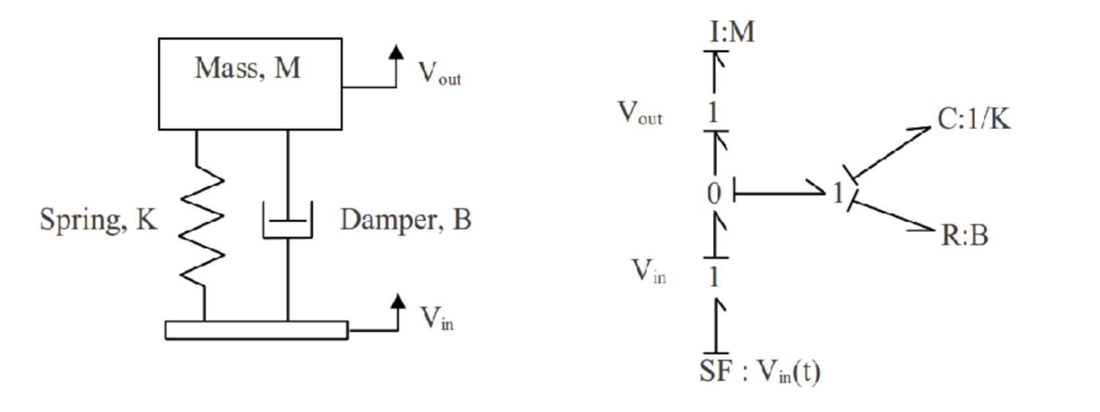
Figure 1: Mechanical Schematic of Quarter Car Model (left) and equivalent bond graph (right).

Dynamic Equations

After a bond graph is created, the first order linear ordinary differential equations that describe how the dynamics of the system change with respect to time can be formulated. You will learn how to generate these equations from a bond graph in this class. For now, we provide you with the resulting two differential equations:

\begin{align*} \dot{p}(t) = K q(t) + B \left(v_{in}(t) - \frac{p(t)}{M}\right) \\ \dot{q}(t) = v_{in}(t) - \frac{p(t)}{M} \end{align*}

These equations define expressions for the derivatives of the two state variables \(p(t)\) and \(q(t)\) which are described below. Note that the time derivatives are the only thing on the left hand side of the equations. This form is called the explicit form, i.e. there are no time derivatives on the right hand side.

The road motion will be described by its vertical velocity (see below "Inputs") but it will also be useful to see what the bump looks like in terms of vertical displacement. To do so, an additional, optional, differential equation can be added. If we know \(v_{in}\) we must integrate to get \(y_{in}\) thus:

\begin{equation*} \dot{y}_{in}(t) = v_{in}(t) \end{equation*}

These three differential equations define the time derivatives of the three state variables which are:

Momentum of the sprung mass: \(p(t)\)
Change in displacement between the sprung mass and the ground: \(q(t)\)
Vertical displacement of the road: \(y_{in}(t)\)

Initial Conditions

Initial conditions are the starting point values for the integrated variables in the systems. This system has three state variables, so there are three initial conditions. For this lab, all the initial conditions are zero. See Integrating the State Equations for how to set up the initial condition vector. Make sure that your initial conditions are arranged in the same order as your state variables.

Parameters

This model has three constant parameters associated with the three components. Values for these parameters that represent a light car are:

Quarter car mass: \(M = 267 \textrm{ kg}\)
Linear shock absorber damping coefficient: \(B = 1398 \textrm{ Nsm}^{-1}\)
Linear spring stiffness: \(K = 1.87\times 10^4 \textrm{ Nm}^{-1]}\)

Inputs

We want the velocity input \(v_{in}\) input to represent a triangular bump for the wheel to move over. Since we're describing the velocity input, not displacement, it will take the form of two steps: moving upward for a time, then downward at the same rate for the same duration. Integrating a constant gives a sloped line, i.e. \(\int c dx = cx\). Start with an amplitude of the step as \(A = 0.2 \textrm{ms}^{-1}\) and the steps described by:

\begin{equation*} v_{in}(t) = \begin{cases} A & \text{if}\ 0.5s \leq t < 1.0s \\ -A & \text{if}\ 1.0s \leq t < 1.5s \\ 0 & \text{otherwise} \\ \end{cases} \end{equation*}

Outputs

A suspension designer may be interested in knowing how much force the spring and damper are expected to experience, so that they can size the components appropriately. The forces can be determined from a force balance:

\begin{align*} F_{spring}(t) = K q(t) \\ F_{damper}(t) = B \left(v_{in}(t) - \frac{p(t)}{M}\right) \end{align*}

A designer concerned with the comfort of the passengers may like to know what the maximum absolute vertical acceleration is of the vehicle. The acceleration is a function of the time derivative of a state variable:

\begin{equation*} a(t) = \frac{\dot{p}(t)}{M} \end{equation*}

Time Steps

You will also have to decide on how long your simulation will run and at what time resolution you should report values of the states, inputs, and outputs. To help in deciding on computing time steps and the total time for a computing run, it is useful to compute natural frequencies and damping ratios.

The natural frequency of this system is:

\begin{equation*} \omega_n = \sqrt{\frac{K}{M}} \end{equation*}

This can be expressed in cycles per second (Hertz) instead of radians per second with:

\begin{equation*} f_n = \frac{\omega_n}{2\pi} \end{equation*}

The damping ratio of this system is defined as:

\begin{equation*} \zeta = \frac{B}{2\sqrt{MK}} \end{equation*}

Use these values to determine how long your simulation should last such that at least five oscillations occur or the oscillation magnitude is reduced to approximately 1/10 maximum. Also use them to choose a time resolution (spacing between time steps) such that you plot at least ten time points for the shortest duration oscillation.

Deliverables

Submit a report as a single PDF file to Canvas by the due date that addresses the following items:

Create a function defined in an m-file that evaluates the right hand side of the ODEs, i.e. evaluates the state derivatives. See Defining the State Derivative Function for an explanation.
Create a function defined in an m-file that generates the bump in the road. See Time Varying Inputs for an explanation.
Create a function defined in an m-file that calculates two outputs: force applied to the damper and force applied to the spring. See Outputs Other Than the States for an explanation.
Create a function defined in an m-file that calculates the vertical acceleration. See Outputs Involving State Derivatives
Create a script in an m-file that utilizes the above four functions to simulate the suspension system traversing the bump in the road. This should setup the constants, integrate the dynamics equations, and plot each state, input, and output versus time. See Integrating the State Equations for an explanation.
Show the effects that removing the damper, i.e. setting \(B=0\), has on traversing the bump. Use plots and written text to describe the differences in the motion.
Choose one of the following road inputs and create an m-file that generates this input:
1. A sinusoidal undulating road input with velocity amplitude of 0.1 meters per second, at the natural frequency: \(\sqrt{K/M}\).
2. Driving over a 20 cm curb.
3. A random roadway with bumps described by a velocity input uniformly distributed between -0.1 and 0.1 meters per second.
Plot the resulting simulation and describe the motion and what you learn from it.

Notes On Creating A Quality Submission

Include a title page with the lab assignment name & number, course, quarter, year, date, your name, and student ID.
Use both text and plots to explain your work and findings.
Include your code in the report. Show each function and the main script. These should be monospaced font formatting and ideally syntax highlighted. You can use the publish function in Octave and Matlab to export code files to nice formats. See https://www.mathworks.com/help/matlab/matlab_prog/publishing-matlab-code.html for more information.
Your code should be readable by someone else. Include comments, useful variable names, and follow good style recommendations, for example see this guide. Imagine that you will come back to this in 10 years and you want to be able to understand it quickly.
All functions should have a "help" description written in the standard style describing the inputs and outputs of the function. This template is useful (click the function tab).
All plots should have:
- Axes labeled with units
- Axes limits set to show the important aspects of the graph
- Fonts large enough to read (>= 8pt)
- A figure number, short title, and caption explaining what the figure is
- Legends to describe multiple lines on a single plot