Contents
Learning Objectives
After completing this lab you will be able to:
- translate ordinary differential equations into a computer function that evaluates the equations at any given point in time
- numerically integrate ordinary differential equations with Octave/Matlab's ode45
- create complete and legible plots of the resulting input, state, and output trajectories
- create a report with textual explanations and plots of the simulation
- explain how various parameters affect the motion of a two degree-of-freedom quarter car model
Introduction
In the last lab, you simulated a one degree-of-freedom quarter car suspension model. Here we present a two degree-of-freedom quarter car suspension model in which the additional degree-of-freedom captures the simplified compression/extension of the tire between the wheel hub and the ground. Similar to the prior lab, the goal is to simulate this system to see the response as it is driven over a pothole.
To view the system response to driving over a pothole, you need to:
- Determine the state equations, states, constant parameters, inputs, initial conditions, and outputs.
- Write the functions for calculating the state derivatives, inputs, and outputs.
- Simulate the system and plot the desired responses.
- Interpret and explain the results.
Model Description
The sprung mass, \(M\), represents a quarter of the weight of the car that is located above the shock absorber. The shock absorber is represented by a linear spring and damper in parallel. The unsprung mass, \(M_u\), represents the mass of the wheel and tire. The spring between the unsprung mass and the ground represents the stiffness of the tire. Power flowing from the system to the ground is considered positive (note the direction in which positive velocity is defined).
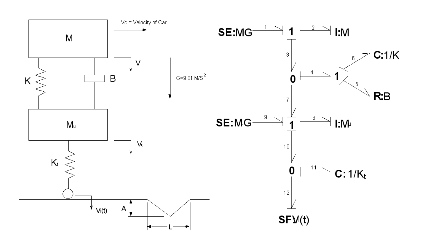
Figure 1: (left) schematic of the two degree-of-freedom quarter car model and (right) a bond graph representing the system
State Equations and States
The state equations derived from the bond graph are as follows:
where the time varying states are defined as:
- \(p_2\): vertical momentum of the sprung mass [kg m/s]
- \(q_6\): displacement between the sprung and unsprung mass [m]
- \(p_8\): vertical momentum of the unsprung mass [kg m/s]
- \(q_{11}\): displacement between the unsprung mass and the ground [m]
It will once again be useful to find the vertical displacement of the road, \(y_i\) [m], to visualize the shape of the road. An additional state equation and state \(y_i\) can be added to the above minimal set of equations to calculate the road height. You have to add this as a state equation and not an output equation because it requires integration to compute.
Constant Parameters
The quarter car is defined by the following constant parameters:
- Sprung mass: \(M = 250 \textrm{ kg}\)
- Ratio of the sprung and unsprung masses: \(\frac{M}{M_u} = 5\)
- Acceleration due to gravity: \(g=9.81 \textrm{ ms}^{-2}\)
- Natural frequency of the sprung mass: \(f_n=1 \textrm{ Hz}\)
- Damping ratio of the sprung mass: \(\zeta=0.3\)
- Ratio of the tire and suspension spring stiffnesses: \(\frac{K_t}{K} = 10\)
The pothole input is defined by the following constant parameters:
- Forward speed of the car: \(V_c = 10 \textrm{ ms}^{-1}\)
- Width of the pothole: \(L = 1.2 \textrm{ m}\)
- Depth of the pothole: \(A = 0.08 \textrm{ m}\)
Initial Conditions
The initial velocities of the two masses should be set to zero, which implies that the momentums are also zero:
The initial conditions of the displacements, \(q_6,q_{11}\), should reflect the equilibrium state of the springs. To find the equilibrium value of the two displacements, set the momentums, their time derivatives, the time derivatives of the displacements, and the road velocity input equal to zero in the state equations and solve for \(q_6,q_{11}\). Use these results as the initial conditions.
Inputs
The single input to the model is the vertical velocity of the road \(v_i\) as seen from a reference frame that translates with the forward motion of the car. This velocity will vary over time and be partially determined by the travel speed of the car.
When the wheel hits the first part of the pothole, the wheel travels down (positive for the bond graph) with a constant vertical velocity. Once the tire reaches the bottom of the hole the wheel reverses its vertical direction and travels up at the same speed. Assume that the profile of the pothole represents the displacement of the point where the tire rubber meets the road. At the end of the pothole, the wheel resumes a vertical velocity of zero.
The amount of time it takes for the tire to cross the pothole is \(T=\frac{L}{v_c}\). Consequently, if the tire enters the pothole at \(t=T_1\), the middle of the pothole occurs at \(T_2 = T_1 + T/2\), and the tire leaves the pothole at \(T_3 = T_1 + T\). The vertical velocity is given by \(v_i = v_c\frac{dy}{dx}\), where \(\frac{dy}{dx}\) is the slope of the pothole. Using the slope, you can find an equation for the amplitude of the velocity input. You will need to create a function that calculates this input for any given time, \(t\).
Outputs
One output that may be useful for a suspension engineer is the deflection of the suspension relative to the equilibrium deflection. You may know that if the suspension bottoms out, there may be damage to the car when hitting the pothole. The deflection of the suspension is:
Remember a positive number represents compression. Include this output in your report and be sure to discuss what you learn from it.
Another output that is useful is the sprung mass acceleration, as this acceleration will correlate to the forces the car's frame and the passengers experience. Include this output and explain what you learn from it.
Time Duration and Resolution
You need to determine the desired maximum time step to ensure that the simulation outputs capture all important variations with respect to time. To determine the time step you need to think about the dynamics of the system. Useful values to help you do so are the natural frequency and damping ratio of the masses. For example, the natural frequency of the sprung mass is:
This gives you an estimate of the oscillation frequency of the system. Note that you have two springs, each with different natural frequencies. You can calculate the natural period of each to get an idea of the minimum time resolution you may need.
The damping ratio of the sprung mass is:
For an over damped system, this gives you an estimate of of how fast the oscillations will exponentially decay. Remember that the decay function takes this form:
You can figure out the time it takes to decay a particular percentage from this equation. Popular times to check are "time to half" or calculating the time constant \(\tau\), which is the time it takes to decrease 63%. The time constant is defined as:
If the system oscillates very rapidly you will want a shorter time step. If the oscillation is very slow or if there is a huge amount of damping, the time step can be longer. Ensure that there are at least 10 data points per oscillation for the shortest duration period you determine. Also, ensure that the total duration of the simulation includes data up to a decay of \(2\tau\) seconds. Finally, inspect the simulation results and if you think that time resolution doesn't show enough detail in parts of the motion, decrease the time step until it does show sufficient detail. Be sure to explain what you choose and why.
Deliverables
Submit a report as a single PDF file per group to Canvas by the due date that addresses the following items. The report should follow the report template and guidelines.
- Create a function defined in an m-file that evaluates the right hand side of the ODEs, i.e. evaluates the state derivatives. See Defining the State Derivative Function for an explanation.
- Create a function defined in an m-file that generates the pothole in the road. See Time Varying Inputs for an explanation.
- Create a function defined in an m-file that calculates the two outputs: suspension deflection and sprung mass acceleration. See Outputs Other Than the States and Outputs Involving State Derivatives for an explanation.
- Create a script in an m-file that utilizes the above functions to simulate the suspension system traversing the pothole in the road. This should setup the constants, integrate the dynamics equations, and plot each state, input, and output versus time. See Integrating the State Equations for an explanation.
- From the plots above give your best estimation of the vibration period and the frequency of the system. Explain how you determined these numbers.
- Try changing only the damping ratio, \(\zeta\), to a larger and smaller value. Plot suspension deflection and acceleration for these new damping ratios. What happens when \(\zeta\) decreases/increases? How does the change in \(\zeta\) affect the mass acceleration?
Assessment Rubric
Points will be added to 40 to get your score from 40-100.
Functions (10 points)
- [10] All functions (1 state derivative, 1 input, 1 output) are present and take correct inputs and produce the expected outputs.
- [5] Most functions are present and mostly take correct inputs and produce the expected outputs
- [0] No functions are present.
Main Script (10 points)
- [10] Constant parameters only defined once in main script(s); Integration produces the correct state, input, and output trajectories; Good choices in number of time steps and resolution are chosen and explained
- [5] Parameters are defined in multiple places; Integration produces some correct state, input, and output trajectories; Poor choices in number of time steps and resolution are chosen or not explained
- [0] Constants defined redundantly; Integration produces incorrect trajectories; No clear choices in time duration and steps
Explanations (10 points)
- [10] Explanation of damping effects is correct and well explained; Explanation of the vibration period and frequency is correct and well explained; Plots of appropriate variables are used in the explanations
- [5] Explanation of damping effects is somewhat correct and reasonably explained; Explanation of vibration period and frequency is somewhat correctly describes results; Plots of appropriate variables are used in the explanations, but some are missing
- [0] Explanation of damping is incorrect and poorly explained; Explanation of vibration and frequency behavior incorrectly describes results; Plots are not used.
Report and Code Formatting (10 points)
- [10] All axes labeled with units, legible font sizes, informative captions; Functions are documented with docstrings which fully explain the inputs and outputs; Professional, very legible, quality writing; All report format requirements met
- [5] Some axes labeled with units, mostly legible font sizes, less-than-informative captions; Functions have docstrings but the inputs and outputs are not fully explained; Semi-professional, somewhat legible, writing needs improvement; Most report format requirements met
- [0] Axes do not have labels, legible font sizes, or informative captions; Functions do not have docstrings; Report is not professionally written and formatted; Report format requirements are not met
Contributions [10 points]
- [10] Very clear that everyone in the lab group contributed equitably. (e.g. both need to do some coding, both work on bond graph, both should contribute to writing)
- [5] Need to improve the contributions of one or more members
- [0] Clear that everyone is not contributing equitably