Contents
Learning Objectives
After completing this lab you will be able to:
- translate ordinary differential equations into a computer function that evaluates the equations at any given point in time
- numerically integrate ordinary differential equations with Octave/Matlab's ode45
- create complete and legible plots of the resulting input, state, and output trajectories
- create a report with textual explanations and plots of the simulation
- explain how various parameters affect the motion of a four degree-of-freedom motocross motorcycle model
Introduction
In this lab, you will investigate the response of a motocross motorcycle as it traverses two road bumps. You will look into the pitch and heave motion of the motorcycle when it travels over the bumps. You will also consider how the rider can change the dynamics of the vehicle by shifting his or her weight for and aft on the motorcycle.
Model Description
The schematic for the model is shown in Figure 1. There is a primary mass and inertia that represents the rider and the motorcycle lumped as a single rigid body supported by front and rear suspension systems and tires.
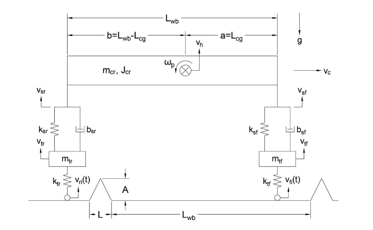
Figure 1 Motocross motorcycle pitch-heave model. In this schematic, the front wheel has already gone over the first bump.
The kinematics are:
with \(a=L_{cg}\) and \(b=L_{wb}-L_{cg}\), \(\theta=\int_0^t\omega_p dt\).
With a small angle assumption in the rotation, this simplification can be used:
System Equations
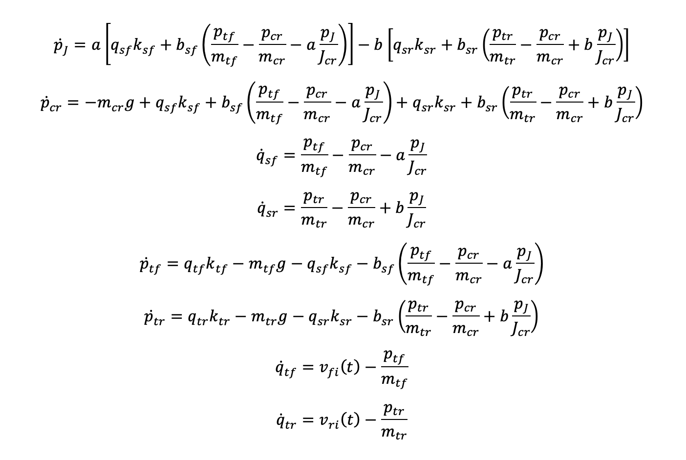
Figure 2 System equations
State Variables
There are eight state variables for the four degree of freedom model.
| \(p_J\) | Pitch angular momentum |
| \(p_{cr}\) | Vertical momentum of motorcycle and rider |
| \(q_{sf}\) | Front suspension spring displacement |
| \(q_{sr}\) | Rear suspension spring displacement |
| \(p_{tf}\) | The momentum of front tire mass |
| \(p_{tr}\) | The momentum of rear tire mass |
| \(q_{tf}\) | Front tire deflection |
| \(q_{tr}\) | Rear tire deflection |
Constant Parameters
| Symbol | Description | Value | Units |
| \(v_c\) | Motorcycle forward velocity | 10 | m/s |
| \(L_{cg}\) | Center of gravity distance (standard config.) | 0.9 | m |
| \(L_{cg}\) | Center of gravity distance (forward config.) | 0.7 | m |
| \(m_{cr}\) | Mass of cycle and rider | 300 | kg |
| \(r_{gy}\) | Body radius of gyration | 0.5 | m |
| \(k_{sf}\) | Front suspension stiffness | 3000 | N/m |
| \(k_{sr}\) | Rear suspension stiffness | 3500 | N/m |
| \(b_{sf}\) | Front damping coefficient | 400 | Ns/m |
| \(b_{sr}\) | Rear damping coefficient | 500 | Ns/m |
| \(m_{tf}\) | Front tire (unsprung) mass | 15 | kg |
| \(m_{tr}\) | Rear tire (unsprung) mass | 20 | kg |
| \(k_{tf}\) | Front tire stiffness | 30,000 | N/m |
| \(k_{tr}\) | Rear tire stiffness | 40,000 | N/m |
| \(L_{wb}\) | Wheel base distance | 1.6 | m |
| \(A\) | Bump height | See Note | m |
| \(L\) | Bump distance | 0.5 | m |
| \(g\) | Acceleration due to gravity | 9.81 | \(\frac{m}{s^2}\) |
| \(\delta_{max}\) | Maximum suspension deflection | 0.1 | m |
The moment of inertia of the motorcycle and rider can be estimated with:
Inputs
Define all system inputs for the effort and flow sources in an input function that returns the five inputs at any given time. The effort sources are the force due to gravity on the tire masses and the mass of the cycle and rider. The flow sources are the road input velocities, dependent on the road profile.
| \(m_{cr}g\) | Gravitational force on cycle and rider |
| \(m_{tf}g\) | Gravitational force on the front tire |
| \(m_{tr}g\) | Gravitational force on the rear tire |
| \(v_{fi}(t)\) | Vertical velocity at the front tire |
| \(v_{ri}(t)\) | Vertical velocity at the rear tire |
The motorcycle will traverse two bumps, each of height \(A\). You need to first define a start time (when the front tire first hits the bump). Then, using the forward velocity and the given cycle/road geometry, find the following:
- The times when the front tire reaches the apex and end of the first bump.
- The times when the front tire reaches the start, apex, and end of the second bump.
- The times when the rear tire reaches the start, apex, and end of the first bump.
- The times when the rear tire reaches the start, apex, and end of the second bump.
- The input velocity amplitude when going up and down a bump (the amplitude is the same for both bumps and for front and rear inputs)
Note: You can assume that the horizontal distance between the wheel bases (\(L_{wb}\)) does not change as the angle of the top mass changes. Show the complete input equations in your report.
You will also need to determine the largest bump height \(A\) which the motorcycle can go over without bottoming out either the front or rear suspension. Bottoming out means that the suspension deflection has equaled or exceeded the maximum suspension deflection. The maximum suspension deflection relative to equilibrium conditions is \(\delta_{\max}=0.1\:m\) for both the front and rear suspensions. The max bump height should be determined for both loading configurations (\(L_{cg}=0.9\textrm{m}\) and \(L_{cg}=0.7\textrm{m}\)).
A clue to determining the max bump height is that the motorcycle model is a linear system, which means that if inputs are scaled up or down, the responses of all variables will be scaled identically (e.g., if you double the inputs, the outputs are doubled as well). This means that only two simulation runs are necessary to determine the size of the bump that will cause the suspension to bottom out (one for each configuration). You may want to use the MATLAB/Octave command max() to find the maximum suspension deflections.
Initial Conditions
You will need to calculate all of the displacements at the equilibrium state and use these values for the initial displacements. Determine the initial conditions from the equations of motion (remember, the system is initially in equilibrium, with all state derivatives equal to zero) or by using statics. Note that it is easiest to define the system of equations and then to use Matlab/Octave's ability to solve systems of equations to calculate the equilibrium values.
Simulation
Simulate the system to obtain the front and rear suspension deflections, heave velocity (vertical velocity of the cycle and rider), and pitch angular velocity. Suspension deflection is defined as the spring displacement minus the initial value so that it starts at zero in gravitational equilibrium.
Time
Set your time control parameters. The time control parameters are the maximum step size and the finish time. To determine these, you will need to estimate the system natural frequencies. Use Figure 3 to approximate the range of natural frequencies for this system.
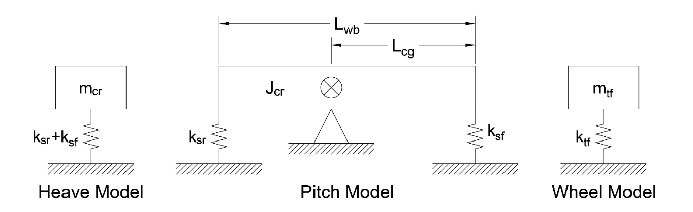
Figure 3 Three independent systems that you can calculate natural frequencies for.
Invert the frequency estimations to determine the vibration periods, and then choose appropriate time parameters. You want the maximum step size to be at most about one-tenth of the shortest vibration period or one-tenth of the time it takes to go over one half of one bump, whichever is shorter. Set the finish time to be about three of the longest vibration periods after the rear tire reaches the end of the second bump. Once you have determined your final time and your step size, set the simulation timespan in the primary script. The following relationships can help you make your calculations:
You may use a small angle assumption (\(\sin\theta\approx\theta\)) when determining the pitch natural frequency.
Deliverables
In your lab report, show your work for creating and evaluating the simulation model. Include your bond graph drawing and any calculations for initial conditions, input equations, maximum bump height, time parameters, and any other parameters. Additionally, provide the indicated plots and answer the questions below. Append a copy of your Matlab/Octave code to the end of the report. The report should follow the report template and guidelines.
Bond Graph
Draw the bond graph for the system with the power flow and velocities as shown in the schematic in Figure 1. Assume spring deflections are positive in compression. Note: when drawing the kinematic relationships between \(v_h,\omega_p,v_{sf},\textrm{ and }v_{sr}\) on the bond graph, use the small angle assumption described above.
Plots
You should provide six total plots, three for the standard center of gravity configuration and three for the forward configuration. For each configuration, provide a plot of:
- The front and rear suspension deflections (on the same plot) versus time.
- The heave velocity versus time.
- The pitch angular velocity versus time.
These plots should be scaled so that the bump size corresponds to the maximum allowable bump height for that center of gravity configuration.
Questions
- What are the natural frequencies of the system? How do these frequencies affect your choice of sample time and simulation length?
- According to the power flow on the bond graph, are the deflections of the suspension positive in compression or tension? Why?
- Compare the plots of the suspension deflections for the two center-of-gravity configurations and describe how the shift in the center of mass affects the system response to the bumps (for example, discuss maximum displacements or shape of the response).
- From the required plots of heave velocity and angular velocity, explain why the spikes in heave velocity are in the same direction, while those of the angular velocity switch direction.
- (Bonus) What would it mean if the force in one of the tires were to become negative (or in other words, if the tire were to be put in tension)? Would the model still be valid? (Hint:Would this happen in real life?) If this is not valid, explain how you would modify your model to make it valid (feel free to try your fix and show results). If you get this correct or show an honest effort in trying to answer this question, you will receive some extra credit.
Code
- Create a function defined in an m-file that evaluates the right hand side of the ODEs, i.e. evaluates the state derivatives. See Defining the State Derivative Function for an explanation.
- Create a function defined in an m-file that generates the five inputs. See Time Varying Inputs for an explanation.
- Create a function defined in an m-file that calculates the necessary outputs. See Outputs Other Than the States and Outputs Involving State Derivatives for an explanation.
- Create a script in an m-file that utilizes the above functions to simulate the suspension system traversing the bumps in the road. This should setup the constants, integrate the dynamics equations, and plot each state, input, and output versus time. See Integrating the State Equations for an explanation.
Assessment Rubric
Points will be added to 40 to get your score from 40-100.
Functions (10 points)
- [10] All functions are present and take correct inputs and produce the expected outputs.
- [5] Most functions are present and mostly take correct inputs and produce the expected outputs
- [0] No functions are present.
Main Script (10 points)
- [10] Constant parameters only defined once in main script(s); Integration produces the correct state, input, and output trajectories; Justified choices in number of time steps and resolution are chosen and explained
- [5] Parameters are defined in multiple places; Integration produces some correct state, input, and output trajectories; Poor choices in number of time steps and resolution are chosen or not explained
- [0] Constants defined redundantly; Integration produces incorrect trajectories; No clear choices in time duration and steps
Explanations (10 points)
- [10] Explanation of dynamics are correct and well explained; Explanation of the vibration period and frequency is correct and well explained; Plots of appropriate variables are used in the explanations
- [5] Explanation of dynamics is somewhat correct and reasonably explained; Explanation of vibration period and frequency is somewhat correctly describes results; Plots of appropriate variables are used in the explanations, but some are missing
- [0] Explanation of damping is incorrect and poorly explained; Explanation of vibration and frequency behavior incorrectly describes results; Plots are not used.
Report and Code Formatting (10 points)
- [10] All axes labeled with units, legible font sizes, informative captions; Functions are documented with docstrings which fully explain the inputs and outputs; Professional, very legible, quality writing; All report format requirements met
- [5] Some axes labeled with units, mostly legible font sizes, less-than-informative captions; Functions have docstrings but the inputs and outputs are not fully explained; Semi-professional, somewhat legible, writing needs improvement; Most report format requirements met
- [0] Axes do not have labels, legible font sizes, or informative captions; Functions do not have docstrings; Report is not professionally written and formatted; Report format requirements are not met
Contributions [10 points]
- [10] Very clear that everyone in the lab group contributed equitably. (e.g. both need to do some coding, both work on bond graph, both should contribute to writing)
- [5] Need to improve the contributions of one or more members
- [0] Clear that everyone is not contributing equitably