1. Introduction to Jupyter

Welcome

Welcome to ENG 122. In this course, we'll be using Jupyter notebooks to experiment with and analyze mechanical systems that vibrate using computation. This first notebook serves as an introduction to the JupyterHub service set up for this class and covers some of the basics of Jupyter notebooks.

After working through this notebook, you will be able to:

• navigate to bicycle.ucdavis.edu to start a JupyterHub notebook server
• open Jupyter notebooks on the JupyterHub and operate the notebook interface
• fetch, validate, and submit assignments
• create well-formatted, fully operational notebooks

Tour de JupyterHub

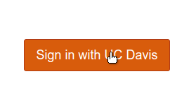
Our computational home for the quarter can be found at bicycle.ucdavis.edu. If you are enrolled in the course, you should be able to log in. Start by clicking the button that says "Sign in with UC Davis".

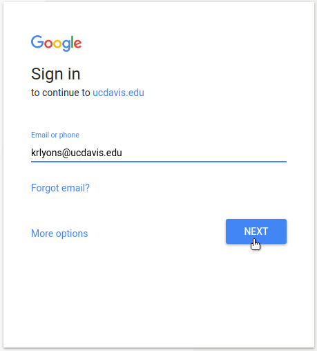
This should direct you to a Google page in which you should enter your UC Davis email.

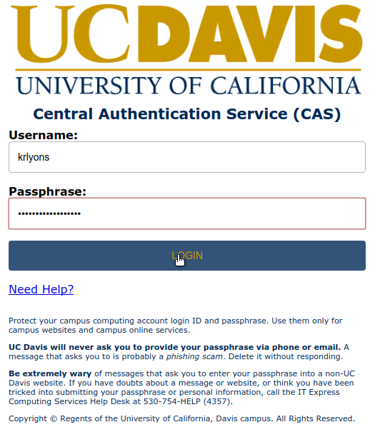
This will in turn direct you to the UC Davis Central Authentication System (CAS). Here, you can enter your UCD username and password.

You're now presented with the Jupyter interface. This is the screen from which you will create notebooks, launch existing notebooks, and work with assignments.

Fetching Notebooks

Let's start by getting ahold of this very notebook so you can open it, modify it, and submit it during class.

1. Go to the "Assignments" tab near the top of the Jupyter interface.
2. Under the "Released assignments" section, you should see eng122_cw01. Go ahead and fetch this assignment.
3. Now there are two ways to open the notebooks in this assignment.
   1. If you go back to the "Files" tab of the Jupyter interface, you should see a folder named eng122_cw01 which contains the fetched notebooks.
   2. Alternatively, you can see the notebooks from the "Assignments" tab in the "Downloaded assignments" section. NOTE that you will need to refresh your browser before the new folder appears on your "Files" tab.
4. Go ahead and open up the notebook eng122_cw01/01-intro-jupyter.ipynb and navigate to this point.

---

Notebook Basics

Working with Cells

Throughout the course, we will be using Jupyter notebooks to perform, demonstrate, and explain computational analyses of vibrational systems. These notebooks are a nice medium for this kind of work because they display and run the analysis code, allow for rich text formatting including nicely typeset equations, and enable interactive plotting. Let's walk through some of the main features of the notebook to get started.

Notebooks are made up of cells, of which there are a couple different types. Markdown cells handle text, equations, and images. Code cells handle Python code. These four elements--text, equations, images, and code--are the four ingredients that constitute a notebook.

What you're reading now is a Markdown cell. You can select a Markdown cell by clicking on it once--you should see a blue border around the cell indicating it is selected.

With a cell selected (blue border), you can insert a new cell below by clicking the plus icon () at the top of the notebook interface or by pressing the "b" key. Go ahead and try it. You can also delete a cell by selecting it and clicking the scissors icon () or pressing the "x" key.

By default, the type of cell that's added is a code cell, which we'll talk about a bit more later. You can change the type of a cell by selecting it and then selecting "Markdown" in the dropdown box near the top of the notebook interface. A nifty keyboard shortcut for changing a cell to Markdown is to press "m".

Note: You can view all of the keyboard shortcuts available by clicking the keyboard icon () at the top of the notebook interface.

You can rearrange the order of cells using the arrow buttons ( and ).

Notebook Ingredient 1: Text

All of the cells you've seen so far have been Markdown cells. What you're looking at now is the Markdown cell after it has been run by clicking the "run cell" button () or using a keyboard shortcut like Ctrl-Enter. To see the source of this cell and to edit its contents, double-click on it or select it and hit Enter. Now you should see that to make bold text, you surround it with two asterisks **.

Here are a few other things you might want to do in a Markdown cell. Remember you can edit a cell to see how these things are achieved.

Bulleted lists:

• bulleted lists can use several different characters to denote an item
• hyphens -
• asterisks *
• plus signs +

Enumerated lists:

1. enumerated lists
2. use numbers

Headings are denoted with one or more # symbols. Using these headings is helpful for structuring a notebook and making it clear that sections are nested within one another.

Math

Another nice feature of Markdown cells is that you can typeset mathematical expressions. The syntax for writing equations is based on LaTeX (pronounced "LAH-tek" or "LAY-tek"). You can write LaTeX in the middle of a sentence (inline) by surrounding it with single dollar signs, for example the text "$Ax = \lambda x$" produces $Ax = \lambda x$. You can also place an equation on its own line (displayed) by putting it on a new line and surrounding it with double dollar signs.

$$e^{i\pi} + 1 = 0$$

A few LaTeX tips:

• Greek letters start with a backslash and are spelled out, e.g. $\delta$
• capital Greek leters are the same but capitalized, e.g. $\Delta$
• fractions use a syntax like \frac{numerator}{denominator}, e.g. $\frac{1}{n}$
• use \cos{}, \sin{}, etc. for $\sin{\theta}$, otherwise it looks like $sin(\theta)$
• integrals $\int x^2 dx$, and with limits $\int_0^\infty e^{-x} dx$
• surround exponents and subscripts with curly brackets {} or only the first character will be raised/lowered, e.g. $e^{ax}$ vs. $e^ax$

Some additional resources:

• https://en.wikibooks.org/wiki/LaTeX/Mathematics
• https://meta.wikimedia.org/wiki/Help:Displaying_a_formula

Images

As shown above with the screenshots of logging in to the JupyterHub server, you can display images in a notebook using the syntax

markdown
![alt text here](path/to/image_file.ext)

or using HTML directly, like

<img src="path/to/image_file.ext" alt="alt text here"/>

If you want to include any hand-written content in your notebooks to help illustrate your analysis in an assignment, you can upload the image file to the JupyterHub server and include it in your notebook as above.

If you have a tablet or touch screen, the simplest option is to use freehand drawing software like Krita to create an image file.

If you would like to put some extra effort in, you can use a vector graphics program like Inkscape to create professional-quality figures. The best way to include these types of graphics is to save in SVG format and include them directly. You can also save it as a rastered format (PNG preferred).

A third option is to draw neatly on paper and take a good photo or scan. By "good," a couple things are implied about the end result (i.e. what you see in the notebook): it is legible and it is understandable. When taking a photo of a drawing, take into account the angle you take the photo from, the lighting, and the image resolution.

To upload an image to the server, you can go into the assignment folder, click the "Upload" button, locate the file on your computer, click the blue "Upload" button, and then include the file in your notebook.

Code

The other type of cell we'll be using extensively is the code cell. This is the default cell type that is added when you click the plus icon near the top of the notebook interface to insert a new cell. Here's an example:

print('hello')

hello

Click somewhere on the above cell so that it is outlined in green and then run it (use the run cell button or hit Ctrl+Enter). Notice that:

• Some output has been generated and displayed below the cell. This is great because the results of your code are now contained in the notebook and when you save the notebook, the output is saved as well.
• The text to the left of the cell used to be In [ ]:, and now there's a number between the square brackets. This indicates that the cell has been run and the number indicates the order of code cell execution in the notebook.

Wrapping Up

The key to creating a notebook that efficiently conveys your thoughts about an engineering problem is to leverage each of these four ingredients for their strengths. For example, a detailed paragraph describing a system with complicated geometry is not nearly as efficient as an image of the system annotated with angles and measurements. In addition, numerical code may not be a great way to demonstrate all of your modeling assumptions for a system.

In general, you should consider how well someone else (or maybe future you) could understand your notebook without the benefit of being in your head.

That's about all we need to know about working with notebooks for now. There are quite a few additional features and tricks that may be shown throughout the course, but the best way to become familiar with notebooks is to use them!

For a bit more comprehensive introduction, see the Jupyter notebook documentation and these introductory examples.

A Few Last Tips

You'll see near the title of your notebook some text that indicates whether or not your notebook contains unsaved changes or if it has autosaved your progress. Even though Jupyter notebooks have autosave functionality, make it a habit to save your notebooks periodically by pressing the save button () or pressing Ctrl+s.

Let's go back to the main Jupyter interface for a minute. If you go to the "Files" tab and navigate to the folder containing this notebook, you'll see that this notebook has a green icon next to it (). If you switch to the "Running" tab, you'll see the full list of notebooks you have running. Even if you close the web browser tab holding a notebook. the notebook remains running in the background.

If you notice that your notebooks are running slowly, check to see how many notebooks you have running in the background and shut down ones you don't need to be running. It may also be a good habit to start closing your notebooks by going to File -> Close and Halt instead of just closing the web browser tab.

Submitting Notebooks

We're done with this notebook, so it's time to submit it. Click the "Kernel" menu and then click "Restart & Run All". It is very important that you do this every time you're finished with a notebook and you're ready to submit it. This will rerun your entire notebook from top to bottom. Once that is finished, make sure all of the outputs look correct. Sometimes, you may find that in interactively working back and forth between cells you introduce some bugs that cause the notebook to fail when it is run from scratch.

To submit the notebook, go to the tab in your browser that you launched this notebook from and get to the "Assignments" tab in the Jupyter interface. Now you can click the "Submit" button next to the assignment called eng122_cw01.