Clock Pendulum with Air Drag Damping
This notebook introduces the third fundamental characteristic of vibration: energy dissipation through damping. A compound pendulum system representing a clock pendulum is implemented that allows students to vary the damping parameters and visualize the three regimes of linear damping.
After the completion of this assignment students will be able to:
- understand the concept of damped natural frequency and its relationship to mass/inertia, stiffness, and damping
- state the three fundamental characteristics that make a system vibrate
- compute the free response of a linear system with viscous-damping in all three damping regimes
- identify critically damped, underdamped, and overdamped behavior
- determine whether a linear system is over/under/critically damped given its dynamic properties
- understand the difference between underdamping, overdamping, and crticial damping
Introduction
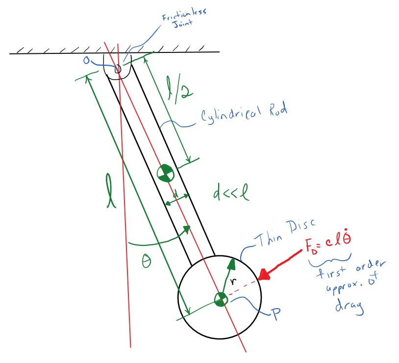
Many clocks use a pendulum to keep time. Pendulum's have a very constant oscillation period and if designed with quality components take very little energy to run. There is a downside to pendulums though. Any friction in the pendulum's pivot joint or any air drag on the pendulum itself will cause the pendulum to slow stop oscillating and this energy dissaption will affect the period of oscillation. resonance includes a simple clock pendulum that represents a clock pendulum that looks like:
Import the pendulum as so:
from resonance.linear_systems import ClockPendulumSystem
sys = ClockPendulumSystem()
Check out its constants. Note that the viscous_damping term is $c$ in the above diagram, i.e. the linear velocity multiplicative factor of the torque due to air drag. Drag is assumed to only act on the bob.
sys.constants
And the coordinates and speeds:
sys.coordinates
sys.speeds
The system can be simulated as usual if the coordinates or speeds are set to some initial value.
import numpy as np
sys.coordinates['angle'] = np.deg2rad(5.0)
traj = sys.free_response(5.0)
And a plot can be shown:
import matplotlib.pyplot as plt
%matplotlib inline
fig, ax = plt.subplots(1, 1)
ax.plot(traj.index, traj.angle)
ax.set_ylabel('Angle [rad]')
ax.set_xlabel('Time [s]');

The above simulation shows that we get a sinusoid oscillation with a period of about 1 second, which is good.
Exercise
Creative an interactive plot of the angle trajectory with a slider for the viscous_damping coefficient. The slider shoudl go from 0.0 to 5.0 with step of 0.1. The code should follow this pattern, as before:
fig, ax = plt.subplots(1, 1)

sim_line = ax.plot(traj.index, traj.angle)[0]
ax.set_ylim((-sys.coordinates['angle'], sys.coordinates['angle']))

ax.set_ylabel('Angle [rad]')
ax.set_xlabel('Time [s]')

def plot_trajectory(viscous_damping=0.0):
    # fill out this function so that the plot will update with a slider.
    # 1) update the system's viscous_damping constant
    # 2) simulate the free response with free_response()
    # 3) update sim_line's data with set_data(x, y)

plot_trajectory()
fig, ax = plt.subplots(1, 1)

sim_line = ax.plot(traj.index, traj.angle)[0]
ax.set_ylim((-sys.coordinates['angle'], sys.coordinates['angle']))

ax.set_ylabel('Angle [rad]')
ax.set_xlabel('Time [s]')

def plot_trajectory(viscous_damping=0.0):
    sys.constants['viscous_damping'] = viscous_damping
    traj = sys.free_response(5.0)
    sim_line.set_data(traj.index, traj.angle)

plot_trajectory()

# write your answer here
from ipywidgets import interact
widget = interact(plot_trajectory, viscous_damping=(0.0, 5.0, 0.1));
Visualize the Motion
sys.constants['viscous_damping'] = 0.2
frames_per_second = 30
traj = sys.free_response(5.0, sample_rate=frames_per_second)
ani = sys.animate_configuration(fps=frames_per_second, repeat=False) # sample time in milliseconds

This is another option for animating that gives a set of play buttons and options.
from IPython.display import HTML
HTML(ani.to_jshtml(fps=frames_per_second))
Exercise
Try out some of the values for the initial coordinate/speed and viscous damping that had interesting trajectories and see what the animation looks like.
Oscillation Period and Viscous Damping
You may have noticed that the period seems to change with different viscous damping values. It is worth investigating this more thoroughly.
Exercise
Use your function for estimating the period of a trajectory in a loop to collect period estimates for 30 values of viscous damping from 0.0 to 5.0. The code for the loop should be structured like:
from resonance.functions import estimate_period

viscous_damping_vals = np.linspace(0.0, 5.0, num=30)
periods = []
for c in viscous_damping_vals:
    sys.constants['viscous_damping'] = c
    # write code here to calculate the period and append to periods
from resonance.functions import estimate_period

viscous_damping_vals = np.linspace(0.0, 5.0, num=30)
periods = []
for c in viscous_damping_vals:
    sys.constants['viscous_damping'] = c
    traj = sys.free_response(5.0)
    periods.append(estimate_period(traj.index, traj.angle))
# write your answer here
fig, ax = plt.subplots(1, 1)
ax.set_xlabel('Damping Coefficient [Ns/m]')
ax.set_ylabel('Period [s]')
ax.set_xlim((0.0, 5.0))
ax.plot(viscous_damping_vals, periods, 'o');

Exercise
Have a look at the periods list and see if anything is unusual. Use the same loop as above but investigate viscous damping values around the value that causes issues and see if you can determine how high the viscous damping value can be for a valid result. The NumPy function np.isnan() can be
for c, T in zip(viscous_damping_vals, periods):
    print('c = {:1.3f}'.format(c), '\t', 'T = {:1.3f}'.format(T))
Reuse both loops from above and calculate viscous_damping values around the location at which the period cannot compute, e.g. 1.55 to 1.65. Maybe use 25 linearly spaced values or so. Find a value for $c$ (viscous_damping) at which the period cannot be computed.
viscous_damping_vals = np.linspace(1.55, 1.65, num=25)
periods = []
for c in viscous_damping_vals:
    sys.constants['viscous_damping'] = c
    traj = sys.free_response(5.0)
    periods.append(estimate_period(traj.index, traj.angle))

for c, T in zip(viscous_damping_vals, periods):
    print('c = {:1.3f}'.format(c), '\t', 'T = {:1.3f}'.format(T))
# write your answer here
Connection to the damping ratio
We defined the damping ratio as:
$$ \zeta = \frac{b}{b_r} = \frac{b}{2m\omega_n} $$sys.constants['viscous_damping'] = 0.2
m, b, k = sys.canonical_coefficients()
b
wn = np.sqrt(k/m)
br = 2*m*wn
br
b / (2*m*wn)
Make a function we can use to calculate the damping ratio:
def calc_zeta():
    m, b, k = sys.canonical_coefficients()
    wn = np.sqrt(k/m)
    return b / (2*m*wn)
Underdamped, $\zeta < 1$
When the viscous damping value is relatively low, a very nice decayed oscillation is present. This is called an underdamped oscillation because there is vibration, but it still dissipates.
Exercise
Create a single plot that shows the free response at these different viscoud damping values: 0.0, 0.08, 0.2, 1.6. Use an initial angle of 5 degrees and inital angular velocity of 0 deg/s. Include a legend so that it is clear which lines represent which values. Use a loop to reduce the amount of typing needed.
fig, ax = plt.subplots(1, 1)

for c in [0.0, 0.08, 0.2, 1.6]:
    sys.constants['viscous_damping'] = c
    traj = sys.free_response(5.0)
    ax.plot(traj.index, traj.angle, label='c = {:0.3f} [Ns/m], $\zeta$ = {:1.2f}'.format(c, calc_zeta()))

ax.legend();

# write your answer here
Critically Damped, $\zeta = 1$
Above in the plot you created of the period of oscillation versus the viscous damping value, you should have discovered that when the value is at 1.6780754836568228 (or somewhere close) that there are no longer any oscillations. This boundary between oscillation and not oscillating wrt to the viscous damping value is called "critically damped" motion.
Exercise
Make a single plot of angle trajectories with the viscous damping value set to 1.67 and an initial angle of 0.1 degrees. Plot three lines with the initial angular velocity as -10 degs, 0 degs, and 10 degrees.
sys.constants['viscous_damping'] = 1.67
sys.coordinates['angle'] = np.deg2rad(0.1)

fig, ax = plt.subplots(1, 1)

for v0 in [-np.deg2rad(10), 0, np.deg2rad(10)]:
    sys.speeds['angle_vel'] = v0
    traj = sys.free_response(5.0)
    ax.plot(traj.index, traj.angle, label='$v_0$ = {:0.3f} [rad/s], $\zeta$ = {:1.2f}'.format(v0, calc_zeta()))

ax.legend()
ax.set_ylabel('Angle [rad]')
ax.set_xlabel('Time [s]')

# write your answer here
Overdamped, $\zeta > 1$
Finally, if the viscous damping value is greater than the critical damping value, the motion is called over damped. There is no oscillation and with very high values of damping the system will rapidly decay.
Exercise
Create a single plot with the viscous damping value at 2.0 and these three sets of initial conditions:
- $\theta_0$ = 1 deg, $\dot{\theta}_0$ = 0 deg/s
- $\theta_0$ = 0 deg, $\dot{\theta}_0$ = 10 deg/s
- $\theta_0$ = -1 deg, $\dot{\theta}_0$ = 0 deg/s
sys.constants['viscous_damping'] = 2.0

initial = ((np.deg2rad(1), 0.0),
           (0.0, np.deg2rad(10)),
           (-np.deg2rad(1), 0.0))

fig, ax = plt.subplots(1, 1)
ax.set_xlabel('Time [s]')
ax.set_ylabel('Angle [deg]')

for x0, v0 in initial:
    sys.coordinates['angle'] = x0
    sys.speeds['angle_vel'] = v0
    traj = sys.free_response(5.0)
    lab_temp = '$x_0$ = {:0.1f} [deg], $v_0$ = {:0.1f} [deg/s], , $\zeta$ = {:1.2f}'
    ax.plot(traj.index, np.rad2deg(traj.angle),
            label=lab_temp.format(np.rad2deg(x0), np.rad2deg(v0), calc_zeta()))

ax.legend();

# write your answer here