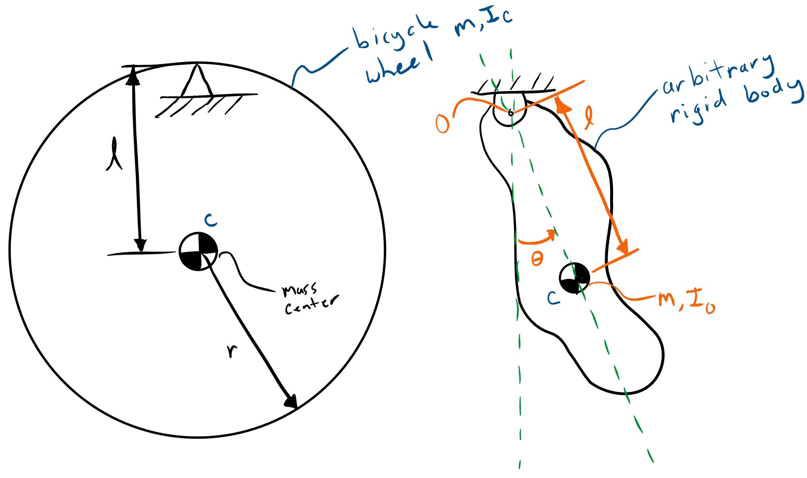
Compound Pendulum and Center of Percussion
At this point we have figured out the moment of inertia about any radial axis that passes through the center of the wheel. We would also like to find the moment of inertia about the wheel's axle, the spin moment of inertia. This moment of interia affects how fast the bicycle wheel can be acelerated and decelerated. We could potentally hang the bicycle wheel on the torsion rod such that the axle's axis aligns with the torsion bar's axis. But there is a simpler way that only requires a fulcrum point and gravity to act as our (constant force) "spring". The video below shows a children's bicycle wheel hanging by the inner diameter of the rim on a small circular rod and a angular velocity gyro is attached to the wheel with it's measurement axis align with the wheel's axle. This arrangement is called a compound pendulum. A compound pendulum is any single degree of freedom pendulum in whch the swinging portion can be considered a rigid body.
from IPython.display import YouTubeVideo
YouTubeVideo('D2tSoGqhtx0', width=640, height=480)
The figure below shows a free body diagram of a compound pendulum. In our case the wheel is the rigid body and the revolute joint is the fulcrum.
The data from the measurement of the same full sized bicycle wheel from the previous analysis can be loaded with:
import pandas as pd
axial_gyro_meas = pd.read_csv('bicycle-wheel-axial-inertia-rate-gyro-measurement.csv',
                              index_col='time')
axial_gyro_meas.head()
axial_gyro_meas.plot(style='.');
Note that this measurement has much less damping than the torsional pendulum. Once again our goal is to determine what the moment of the inertia of the bicycle wheel is. We can use a CompoundPendulumSystem to simulate this motion:
from resonance.linear_systems import CompoundPendulumSystem
cpend_sys = CompoundPendulumSystem()
The compound pendulum system has four constants:
pendulum_mass: mass of the rigid body being swung as a compound penduluminertia_about_joint: the moment of inertia about the fulcrum jointjoint_to_mass_center: the distance from the fulcrum joint to the mass centeracc_due_to_gravity: the acceleration due to gravity
cpend_sys.constants
The mass and radius of the wheel is the same as above. You can get a rough estimate the rotational moment of inertia about the axle as:
$$ I_c = m r^2 $$This assumes that all of the mass is concentrated in a thin ring at the outer most radius, which is not the best estimate but a reasonable value to start with.
But the inertia about the joint has to be computed using the parallel axis theorem.
Exercise
Using the parallel axis thereom, compute an estimate of the inertia about the joint if the distance from the axle to the joint is 0.296 meters. Store both results in variables named inertia_about_axle and inertia_about_joint.
The parrallel axis theorem states that the inertia about any point is equal to the inertia about the mass center plus the total mass times the square of the distance between the point and the mass cetner, i.e.:
$$I_o = I_c + ml^2 $$- $I_o$ is the moment of inertia about a point $o$
- $I_c$ is the moment of inertia about the mass center $c$
- $m$ is the mass of the rigid body
- $l$ is the distance from point c to point o
The mass of the wheel in the video is 1.55 kg and the radius to the outer most portion of the tire is 0.336 m. The distance from the axle to the fulcrum is 0.296 m.
mass = 1.55  # kg
radius = 0.336  # m
inertia_about_axle = mass * radius**2
inertia_about_axle
inertia_about_joint = inertia_about_axle + mass * 0.296**2
inertia_about_joint
# write your solution here
Now simulate the pendulum with an initial angular velocity that is the same as measurement and see how well they match.
cpend_sys.constants
cpend_sys.constants['acc_due_to_gravity'] = 9.81  # m/**2
cpend_sys.constants['inertia_about_joint'] = inertia_about_joint  # kg m**2
cpend_sys.constants['joint_to_mass_center'] = 0.296  # m
cpend_sys.constants['pendulum_mass'] = 1.55  # kg
cpend_sys.speeds['angle_vel'] = axial_gyro_meas.loc[0.0]['angular_velocity']
trajectory = cpend_sys.free_response(5)
import matplotlib.pyplot as plt
%matplotlib inline
fig, ax = plt.subplots(1, 1)
ax.plot(axial_gyro_meas.index, axial_gyro_meas, '.')
lines = ax.plot(trajectory.index, trajectory['angle_vel'])
line = lines[0]

def plot(inertia_about_joint=0.5):
    cpend_sys.constants['inertia_about_joint'] = inertia_about_joint
    traj = cpend_sys.free_response(5)
    line.set_data(traj.index, traj['angle_vel'])

from ipywidgets import interact
interact(plot, inertia_about_joint=(0.0, 1.0, 0.001));
Exercise
Use your decaying_sinusoid function to find a best fit for this data.
import numpy as np
from scipy.optimize import curve_fit
from utils import freq2period, period2freq, decaying_sinusoid
decaying_sinusoid?
popt, pcov = curve_fit(decaying_sinusoid,
                       axial_gyro_meas.index,
                       axial_gyro_meas.angular_velocity,
                       p0=(0.6, -0.0002, 1.0 / 0.44 * np.pi * 2))

ax = axial_gyro_meas.plot(style='.')
ax.plot(axial_gyro_meas.index, decaying_sinusoid(axial_gyro_meas.index, *popt));

# write you answer here
Exercise
The equation of motion for a compound pendulum is:
$$ I_o \ddot{\theta} + mgl\sin\theta = 0 $$For small motions, $\sin\theta\approx\theta$, thus a linearized equation of motion about $\theta=0$ is:
$$ I_o \ddot{\theta} + mgl\theta = 0 $$If the equation of motion can also be written as:
$$ \ddot{\theta} + \omega_n^2 \theta = 0$$Then then a relationship between the period of oscillation and the moment of inertia about the fulcrum joint can be determined.
Write a function of $T$ to caculate $I_o$ based on the above linearized equation of motion and the canonical form which is written in terms of $\omega_n$.
write solution here
Exercise
Finally, using the period of oscillation, $T$, from the data above, you can compute the inertia about the joint using this relationship:
Store the result of this calculation in a variable called actual_inertia_about_the_joint.
# write your solution here
actual_inertia_about_joint = freq2period(popt[2])**2 / 4/ np.pi**2 * mass * 9.81 * 0.296
actual_inertia_about_joint
Exercise
Use the parallel axis thereom to find the moment of inertia about the axle (the location of the center of mass) and store it in a variable called actual_inertia_about_axle. How does this compare to the initial guess of $I_c=mr^2$?
actual_inertia_about_axle = actual_inertia_about_joint - mass * 0.296**2
actual_inertia_about_axle
# write your answer here
Center of Percussion
The center of percussion of a compound pendulum is described as the location on the pendulum that exhibits zero translational acceleration at the pivot joint when an impulse is applied. This corresponds to the length of a simple pendulum of the same mass which has the same frequency of oscillation.
The baseball bat: https://physics.csuchico.edu/baseball/DrBaseball/SweetSpot/
The following video demonstrates the principle:
YouTubeVideo('Dw3UpKQVhVY', width=640, height=480)
Using a SimplePendulumSystem we can simulate it alongside the compound pendulum to determine the center of percussion.
from resonance.linear_systems import SimplePendulumSystem
spend_sys = SimplePendulumSystem()
spend_sys.constants
spend_sys.constants['acc_due_to_gravity'] = 9.81
spend_sys.constants['pendulum_mass'] = 1.55
spend_sys.constants['pendulum_length'] = 0.3
spend_sys.speeds['angle_vel'] = axial_gyro_meas.loc[0.0]['angular_velocity']
spend_traj = spend_sys.free_response(5)
cpend_sys.constants['inertia_about_joint'] = actual_inertia_about_joint
cpend_traj = cpend_sys.free_response(5)
fig, ax = plt.subplots(1, 1)

ax.plot(cpend_traj.index, cpend_traj.angle, label='compound')
lines = ax.plot(spend_traj.index, spend_traj.angle, label='simple')

ax.legend()

def plot(pend_length=0.3):
    spend_sys.constants['pendulum_length'] = pend_length
    spend_traj = spend_sys.free_response(5)
    lines[0].set_data(spend_traj.index, spend_traj.angle)
plot()

interact(plot, pend_length=(0, 1.0, 0.01));