14 Exploring the Motion of a Bicycle
Imports and setup
import numpy as np
import matplotlib.pyplot as plt
from IPython.display import YouTubeVideo
np.set_printoptions(precision=4, linewidth=100)
%matplotlib inline
Introduction
The free response of a bicycle can exhibit vibrational phenomena. If you push a standard bicycle up to speed and then perturb it, it may vibrate. See the following video from the Ruina Lab at Cornell:
YouTubeVideo('pOkDbXEJb8E', width=800, height=600)
One of the simplest models that can predict the fundamental free motion of a bicycle or motorcycle takes the following form:
$$ \mathbf{M\ddot{q}} +v\mathbf{C}_1\mathbf{\dot{q}} +\left[g\mathbf{K}_0 +v^2\mathbf{K}_2\right]\mathbf{q} =\mathbf{F} $$where
$$ \mathbf{q} = [\phi \quad \delta]^T $$$\delta$, the steer angle, is a generalized coordinate that tracks the angle between the front frame (handlebar/fork) and the rear frame (frame, seat, etc) and $\phi$, the roll angle, is a generalized coordinate that tracks the roll angle of the rear frame relative to the ground. If each of these are zero the bicycle is standing upright and the steering is pointed straight ahead. Positive steer angle is to the right and negative steer angle is to the left. Positive roll is to the right and negative to the left.
This model can be constructed by creating an idealized bicycle with four rigid bodies: two wheels, rear frame (main frame and/or rigid person), and front frame (fork/handlebar). The derivation of this model is non-trivial, but you can read about it and more in the 2007 paper: http://rspa.royalsocietypublishing.org/content/463/2084/1955. The following two figures are taken from that paper and are copyrighted to the Royal Society:
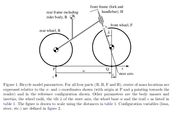
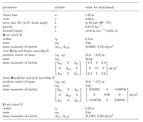
The canonical coefficient matrices are functions of the following 29 constants:
The system has a mass matrix, $\mathbf{M}$, and effective damping and stiffness matrices, $\mathbf{C}=v\mathbf{C}_1$ and $\mathbf{K}=g\mathbf{K}_0 + v^2\mathbf{K}_2$, that are parameterized by the speed of the bicycle $v$ and the acceleration due to gravity $g$. These matrices are a function of the vehicle's geometry and mass distribution.
To work with this model you can load in the BicycleSystem:
from resonance.linear_systems import BicycleSystem
sys = BicycleSystem()
Typical values for the paramers in SI units are (from the above table):
sys.constants
The canonical coefficient matrices are given by:
M, C, K = sys.canonical_coefficients()
M
C
K
Modal Solutions
A damped system will have solutions, in the modal coordinates, that look like:
$$ r_i(t) = A_i e^{-\zeta_i \omega_i t} \sin(\omega_{di} t + \phi_i) $$or
$$ r_i(t) = A_i e^{-\zeta_i t} $$Just like the single degree of freedom systems we have studied. And just like the undamped multi degree of freedom systems, the parameters of this solution are found by calculating the eigenvalues and eigenvectors.
In the actual coordinates the trajectories of the states will look like:
$$ \mathbf{x}(t) = \sum c_i \mathbf{u}_i e^{-\zeta_i \omega_i t} \sin(\omega_{di} t + \phi_i) + \sum c_j \mathbf{u}_j e^{-\zeta_j t} $$Eigenvalues and Eigenvectors
In the previous class we learned that the free response of the system can be formulated by solving an eigenvalue problem. This applies to systems with or without damping. All scientific computing software provides efficient numerical routines to compute the eigenvalues and eigenvectors of a square matrix. In Python you can use numpy.linalg.eig. For systems that have a general damping matric, this computation requires that the system be in state space form. State space form is the explicit first order form of the linear equations where $\mathbf{A}$ is the state matrix and $\mathbf{B}$ is the input matrix.
where $\mathbf{x}$ is the state vector and $\mathbf{r}$ is the input vector.
The transformation from canonical form to state form can be done like so:
$$ \mathbf{x} = \left[\mathbf{q} \quad \mathbf{u}\right]^T = \left[\phi \quad \delta \quad \dot{\phi} \quad \dot{\delta}\right]^T\\ \mathbf{r} = \left[\mathbf{0} \quad \mathbf{F}\right]^T \\ \mathbf{A} = \begin{bmatrix} \mathbf{0} & \mathbf{I} \\ -\mathbf{M}^{-1} \mathbf{K} & -\mathbf{M}^{-1} \mathbf{C} \end{bmatrix}\\ \mathbf{A} = \begin{bmatrix} \mathbf{0} \\ \mathbf{M}^{-1} \mathbf{F} \end{bmatrix} $$Exercise
Write a function that takes the matrices $\mathbf{M,C,K}$ as an inputs and returns the A and B matrices.
def compute_state_matrix(M, C, K):
    """Returns the state matrix.

    Parameters
    ----------
    M : array_like, shape(2,2)
        The mass matrix.
    C : array_like, shape(2,2)
        The damping matrix.
    K : array_like, shape(2,2)
        The stiffness matrix.

    Returns
    -------

    A : ndarray, shape(4,4)
        The state matrix.
    B : ndarray, shape(4,1)

    """

    # write your code here

    invM = np.linalg.inv(M)

    # sub-matrices
    a11 = np.zeros((2, 2))
    a12 = np.eye(2)
    a21 = -invM @ (K)
    a22 = -invM @ (C)

    # note that np.bmat returns a matrix but we don't want that! so make it an array
    A = np.array(np.bmat([[a11, a12], [a21, a22]]))

    B = np.bmat([[np.zeros((2, 2))],
                 [-invM]])

    return A, B
Now use the function to create a state matrix, $\mathbf{A}$, for $v=5.4 \textrm{m/s}$ and $g=9.81$. This speed is normal "around town" riding speed (12 mph).
A, B = compute_state_matrix(M, C, K)
A, B
Now compute the eigenvalues and eigenvectors of the the system using numpy.linalg.eig, see https://docs.scipy.org/doc/numpy/reference/generated/numpy.linalg.eig.html.
eigenvalues, eigenvectors = np.linalg.eig(A)
The eigenvalues are, in general, complex numbers. The complex eigenvalues come in complex conjugate pairs. Each pair corresponds to one osciallatory mode of motion. The real eigenvalues each correspond to one non-osciallatory mode of motion.
eigenvalues
eigenvectors
Plot eigenvectors on polar plot
One way to visualize the modes of motion is by plotting phasor plots of each of the eigenvector components. Eigenvectors are made up of $n$ components, each which may be real or imaginary, that correspond to the states variables. In our case each each component is tied to the roll angle, steer angle, roll angular rate, and steer angular rate. It is also important to note that the phasor plot for osciallation (underdamped) of the derivative of one of the variables simply increases the magnitue by a factor $\omega_i$ and phase shifts the variable by $90^\circ$, i.e.:
$$ r_i(t) = A_i e^{-\zeta_i \omega_i t} \sin(\omega_{di} t + \phi_i) \\ \dot{r}_i(t) = \omega_{di} A_i e^{-\zeta_i \omega_i t} \cos(\omega_{di} t + \phi_i) $$This means that we only need to look at the components associated with the angles to see how the vehicle is moving.
A nice way to plot phasors that are using a polar plot. For example if I have an eigenvalue of $-1.2 + 6j$ that has an associated eigenvector of $[-0.011-0.123j, -0.032-0.149j, 0.581+ 0.067j, 0.789]$ then we can select the first two components and plot a line that is equivlanent to the magnitude of the component and at an angle based on the tangent of the imaginary over the real part.
fig, ax = plt.subplots(1, 1, subplot_kw={'projection': 'polar'})

# this gets the first component of the second eigenvector
v = eigenvectors[0, 1]

radius = np.abs(v)
theta = np.angle(v)

ax.plot([0, theta], [0, radius]);

Exercise
Make polar phasor plots for each of the eigenvalues.
fig, axes = plt.subplots(2, 2, subplot_kw={'projection': 'polar'})

for i, ax in enumerate(axes.flatten()):
    e_val = eigenvalues[i]
    evec = eigenvectors[:, i]
    radius = np.abs(evec[0])
    theta = np.angle(evec[0])
    ax.plot([0, theta], [0, radius], linewidth=2, alpha=0.75)
    radius = np.abs(evec[1])
    theta = np.angle(evec[1])
    ax.plot([0, theta], [0, radius], linewidth=2, alpha=0.75)
    ax.set_title('{:1.3f}'.format(e_val))
ax.legend(['Roll Angle', 'Steer Angle'])
plt.tight_layout()

Animate in the phasors
from resonance.functions import Phasor, PhasorAnimation
times = np.arange(0, 3, 0.03)

i = 0

phasors = [
    Phasor.from_eig(eigenvectors[0, i], eigenvalues[i]),
    Phasor.from_eig(eigenvectors[1, i], eigenvalues[i]),

]

fig = plt.figure()
fig.set_size_inches(3, 6)
ani = PhasorAnimation(fig, times, phasors, repeat=True,
                      re_range=(-0.5, 0.5), im_range=(-0.5, 0.5))

Examine the Mode Shape Trajectories
phi0, delta0, phidot0, deltadot0 = np.real(eigenvectors[:, 0])
sys.coordinates['phi'] = phi0
sys.coordinates['delta'] = delta0
sys.speeds['phidot'] = phidot0
sys.speeds['deltadot'] = deltadot0
traj = sys.free_response(5.0)
traj[['phi', 'delta']].plot(subplots=True);

Exercise
Plot the real part of the eigenvalues as a function of speed and the imaginary part of the eigenvalues as a function of speed. Explain what you learn about the stability of each mode
speeds = np.linspace(0, 10, num=100)

eigenvalues = np.zeros((len(speeds), 4), dtype=complex)
eigenvectors = np.zeros((len(speeds), 4, 4), dtype=complex)

for i, v in enumerate(speeds):
    sys.constants['v'] = v
    M, C, K = sys.canonical_coefficients()
    A, B = compute_state_matrix(M, C, K)
    eigenvalues[i], eigenvectors[i] = np.linalg.eig(A)
fig, axes = plt.subplots(2, 1)

axes[0].plot(speeds, np.real(eigenvalues), 'k.')
axes[0].axhline(0)
axes[0].set_ylim([-10, 10])
axes[1].plot(speeds, np.imag(eigenvalues), 'k.');

axes[1].set_xlabel('Speed [m/s]')

Below is a function that computes the canonical matrices for the bicycle given various geometric and inerital parameters.
Exercises
Remove the gyro effect of the wheels from your model by setting $I_{zz}$ to zero for both wheels. Is your bicycle still stable in some speed range?
Reverse the trail, $c$, (make negative). Is your bicycle still stable in some speed range?
Keep the gyro effect and the positive trail but change the mass distribution of the front fork such that the bicycle is always unstable.
Make a design with negative trail which still shows some stable speed range.