Bicycle Equations Of Motion
Preface
Attempting to derive the equations of motion of the Whipple bicycle model was the trigger which solidified my graduate research topic. I attempted the derivation for my class project in Mont Hubbard’s winter 2006 multi-body dynamics class and struggled with it well into the summer before finally getting a mostly correct answer. After the fact, I realized much of my pain was caused by a single missing apostrophe in my Autolev source code[1]. Luckily another student in the class, Thomas Englehardt, had also derived the equations and helped me debug by sharing his code and going over his methods. Even then, it turned out that my original equations weren’t “exactly” correct and it wasn’t until Luke Peterson joined our lab and got the bicycle dynamics itch did I get the bugs sorted out in my derivation with his help. Conversations and collaboration with Luke have improved the derivation significantly and influence much of what follows. Luke has also continued to improve the derivation with the goal of printing the first compact symbolic result. With careful parameterization and selection of generalized speeds, the non-linear equations may be able to be put into human readable form.
Non-linear Equations of Motion
The Whipple Model is the foundation of all the models presented in this dissertation. This section details derivation of the non-linear equations of motion using Kane’s method [KL85][2]. The non-linear equations of motion are algebraically unwieldy and no one so far has publicly printed them in a form compact enough to print on reasonably sized paper, and certainly not in a form suitable for any in-depth analytical understanding as pointed out in [MPRS07]. My methodology relies heavily on computer aided algebra to do the bookkeeping in the derivation, so I will only describe the necessary details to correctly derive the equations, leaving the algebra, trigonometry and calculus to the computer. The symbolic equations of motion herein were originally developed using Autolev [KL00], a proprietary and now defunct software package for symbolically deriving equations of motion for multi-body systems. I’ve since used the open source software SymPy to derive the equations with the help of the included mechanics package which was developed in our lab to provide a software package suitable for academia with capabilities similar to Autolev[3]. The input code for both software packages are available in the src/eom directory of the dissertation source files.
Model Description
The Whipple Bicycle Model [Whi99] is defined by this set of assumptions:
- The model is made up of four rigid bodies: the rear frame (the main bicycle frame which may or may not include a rigid rider), the front frame (typically the fork and handlebar assembly), and two wheels.
- The bodies are connected to each other by frictionless revolute joints.
- The wheels have knife edges and contact the ground under pure rolling with no side-slip.
- The complete bicycle is assumed to be laterally symmetric.
- The bicycle rolls on flat ground.
[ASKL05], [LS06], and [MPRS07] all provide excellent overviews of the model, its history, and its features.
Unfortunately the word “model” is often ambiguous. I will attempt to be as precise as possible with my wording. For this chapter, I consider a dynamic model, such as the Whipple Bicycle Model, to be equivalent to another dynamic model if at least the minimal set of equations of motions are the same (i.e. they give the same result when evaluated at a particular configuration and state of interest). This implies that the Whipple Bicycle Model linearized about the nominal configuration is a different model than the non-linear Whipple Bicycle Model. I will try to be explicit when discussing the various models.
I will use the following terminology and labels for the four rigid bodies, see Figure 3.2:
- Rear Frame, \(C\)
- The main bicycle frame which may include parts or all of the rider.
- Rear Wheel, \(D\)
- The rear wheel of the bicycle.
- Front Frame, \(E\)
- The fork and handlebar assembly.
- Front Wheel, \(F\)
- The front wheel of the bicycle.
Parameterization
The benchmark derivation of the linear Whipple model [MPRS07] about the nominal configuration uses a non-minimal set of parameters based on typical geometric parameters and inertia definitions using an inertially fixed reference frame in which the \(x\) axis points forward and the \(z\) axis points down, Figure 3.1. The nominal configuration is defined as the configuration when the steering angle is zero and the bicycle is upright with respect to gravity and the ground plane. The parameters presented in [MPRS07] are not necessarily the best choice of parameters, especially when looking at the model from a non-linear perspective, as they are not the simplest set nor a minimal set. For example, the benchmark parameters can be reduced in number by making use of gyrostats, see [Sha08] for an implementation. Choosing a minimum, constant set of parameters can certainly reduce the complexity of the resulting non-linear equations. In this derivation, I use a parameterization with different geometry and inertial definitions to facilitate a more intuitive non-linear derivation, but do not make use of gyrostats to reduce the number of parameters.
Geometry
The geometry of the Whipple model can be parameterized in an infinite number of ways. It is typical and often natural to define the geometry with respect to the descriptions of bicycle geometry used in the bicycle fabrication industry, such as wheel diameter, head tube angle, trail and or rake, Figure 3.1. Choices of parameterizations like these create unnecessary complications when developing the non-linear equations of motion because they are typically defined with respect to only the nominal configuration of the bicycle and are not constant with respect to the system configuration.
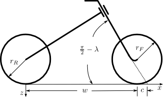
The typical parameterization of the fundamental bicycle’s geometry given in [MPRS07]. The wheelbase \(w\), trail \(c\), steer axis tilt \(\lambda\), front wheel radius \(r_F\), and rear wheel radius \(r_R\) are shown.
With that in mind and after trying various parameterizations, I use geometric formulation presented by [Psi79][4]. The wheels are described by their radius \(\left(r_{F,R}\geq0\right)\) and the remaining geometry is defined by three distances, all of which are configuration invariant. The distance \(d_1\) is the offset to the center of the rear wheel from the steer axis and \(d_3\) is the offset of the front wheel from the steering axis. \(d_2\) is then the distance between the wheel centers as measured along the steer axis. Figure 3.2 gives a complete visual description of the bodies and the geometry.
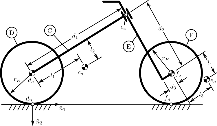
The bicycle in the nominal configuration. The rigid bodies are the rear frame \(C\), rear wheel \(D\), front frame \(E\), and front wheel \(F\). The geometric parameters and important points are also shown.
Generalized Coordinates
The bicycle is completely configured in a Newtonian reference frame by nine generalized coordinates: six coordinates locate and orient the rear frame in space and three additional coordinates are needed for the three revolute joints connecting the front frame and wheels to the rear frame. I made use of the SAE vehicle dynamics reference frame standard and all rotations are are defined as positive right-handed which makes the configuration identical to that in [MPRS07][5]. The rotation matrices are defined as
where \(^n\bar{v}\) is a vector expressed in the \(N\) frame and \(^a\bar{v}\) is the same vector expressed in the \(A\) frame.
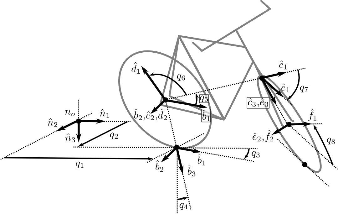
The bicycle in a general configuration showing each of the eight generalized coordinates.
To configure the bicycle, begin by locating the point that follows the rear wheel contact in the ground plane of the Newtonian reference frame, \(N\), with longitudinal and lateral coordinates \(q_1\) and \(q_2\), respectively, see Figure 3.3. Then orient the rear frame, \(C\), with respect to the Newtonian reference frame through a body-fixed 3-1-2 rotation defining the yaw angle, \(q_3\), the roll angle, \(q_4\), and the pitch angle, \(q_5\). The intermediate frames yaw, \(A\), and roll, \(B\), are implicitly generated. The rotation matrix of \(C\) relative to \(N\) is then
where the notation \(s_i = \operatorname{sin}(q_i)\) and \(c_i = \operatorname{cos}(q_i)\) in (2) and also all subsequent equations in this chapter.
The rear wheel, \(D\), rotates with respect to the rear frame about the \(\hat{c}_2\) axis through \(q_6\).
The front frame, \(E\), rotates with respect to the rear frame about the \(\hat{c}_3\) axis through the steering angle, \(q_7\).
Finally, the front wheel, \(F\), rotates with respect to the front frame through \(q_8\) about the \(\hat{e}_2\) axis.
The first two coordinates locate the rear wheel contact point in the Newtonian reference frame and the remaining six coordinates orient the four rigid bodies within the Newtonian reference frame.
The positions of the various points on the bicycle must be defined with respect to the Newtonian reference frame. There are six primary points of interest: the four mass centers, \(d_o,c_o,e_o,f_o\), and the two points fixed on the wheels which are instantaneously in contact with the ground, \(d_n,f_n\)[6].
The mass center of the rear wheel, \(d_o\), is assumed to be at the center of the wheel and is located by
The rear frame mass center, \(c_o\), is located by two additional parameters
For convenience, define an additional point on the steer axis, \(c_e\), such that
The mass center of the front wheel, \(f_o\), is then located by:
The front frame mass center, \(e_o\), is located by two more additional parameters:
The location of the point on the rear wheel instantaneously in contact with the ground in the Newtonian frame is then defined by
The location of the front wheel contact point is less trivial. The vector from the front wheel center to the contact point is defined as
Here the triple cross product divided by its magnitude represents the unit vector pointing from the front wheel center to the point on the front wheel instantaneously in contact with the ground. [BMCP07] give a good explanation and diagram. Another description of this vector is in terms of dot products, i.e. subtract the \(\hat{n}_3\) component of \(\hat{e}_2\) from \(\hat{n}_3\) to get a vector that points from the front wheel center to the contact point.
This is easily shown to be equivalent to (12) by writing the triple cross product as sum of dot products.
Holonomic Constraints
Two holonomic configuration constraints, arising from the fact that both wheels must touch the ground, complicate the model derivation. The first holonomic equation is obviated by definition of the rear wheel center (6). This enforces that the rear wheel contact point cannot have an displacement in the \(\hat{n}_3\) direction[7]. The second holonomic constraint is enforced by requiring the front wheel to touch the ground plane. The constraint is characterized by a non-linear relationship between the roll angle \(q_4\), steer angle \(q_7\) and pitch angle \(q_5\).
In this equation, pitch, \(q_6\), is defined as the dependent coordinate. The choice of pitch has to do with the fact that for “normal” bicycle configurations, pitch is practically constant. This is not universal and it may be smart to choose the dependent coordinate differently for other cases. The constraint equation can actually be formulated into a quartic in the sine of the pitch ([Psi79], [PH08a]) which does have an analytic, albeit lengthy, solution. I do not opt for the analytical solution, so care is needed when simulating and linearizing to properly choose the proper roots associated with this dependent coordinate.
Kinematical Differential Equations
The choice of generalized speeds can significantly reduce the length of the equations of motion [MK96]. This is beneficial for both working with the analytical forms of the equations of motion and the efficiency in computation. Even though this is true, little effort was spent in selecting optimal generalized speeds, as the analytical form of the equations of motion of this system would be difficult to interpret regardless of the choice and because computational speed was of little concern. For \(i=1,\dotsc,8\) simply choose the generalized speeds to be equal to the time derivatives of the generalized coordinates
Velocity
The angular and linear velocities of each rigid body are required for computing the partial velocities and accelerations used in Kane’s method. Also, the velocities of the points on the wheels at the ground contact points are needed for the development of the nonholomic constraints. The angular velocity of the rear frame, \(C\), in \(N\) is
Both the front frame and the rear wheel are connected to the bicycle rear frame by simple revolute joints, so the angular velocities are simply
and
The front wheel has angular velocity relative to the front frame
The angular velocity of any of the bodies can now be computed with respect to the Newtonian reference frame. For example,
which expands to
Using the angular velocities and the position vectors, the velocities of the mass centers can be computed. Starting with mass center of the rear wheel
The remaining velocities can be computed by taking advantage of the fact that various pairs of points are fixed on the same rigid body. The mass centers of the rear wheel, \(d_o\) and the rear frame, \(c_o\), and the steer axis point, \(c_e\), (Figure 3.2) all lie on the rear frame.
where
and
where
The velocity of the front wheel mass center is computed with respect to the steer axis point as they both lie on the front frame
where
Then the velocity of the front frame mass center is similarly
where
The velocity of the contact points on the wheel are needed to enforce the no-slip condition and can be computed with respect to the rear and front wheel centers. The rear contact point is
where
which simplifies to
The front wheel contact velocity is
where
Acceleration
The angular acceleration of each body along with the linear acceleration of each mass center are required to form \(F_r^*\) in Kane’s equations. The angular acceleration of the rear frame, \(C\), in \(N\) is
The remaining bodies’ angular accelerations follow from simple rotations
The linear acceleration of each mass center can then be computed. The acceleration of the rear wheel center of mass is
The remaining accelerations are computed using the analogous two point relationship utilized for the velocities. The acceleration of the rear frame center of mass is
where
and
The acceleration of the steer axis point is
where
and
The acceleration of the front wheel center of mass is
where
and
The acceleration of the front frame center of mass is
where
and
Motion Constraints
Motion constraints reduce the dimensions of the locally achievable configuration space from nine to three. The first four constraints are introduced to enforce the pure rolling, no side-slip, contact of the knife-edge wheels with the ground plane and are nonholonomic. This sets the components of velocity of the contact points on the wheels in the \(\hat{a}_1\) and \(\hat{a}_2\) directions equal to zero, producing the following relationships
The fifth motion constraint is used to enforce the constraint on the velocities imposed by the holonomic constraint, Equation (14). This is strictly introduced to ease numerical integration and linearization. By differentiating the holonomic constraint equation we arrive at an equation that is linear in the generalized speeds and can be treated as any other motion constraint
These five equations are linear in the eight generalized speeds. Following convention, I choose the roll rate, \(u_4\), the rear wheel rate, \(u_6\), and steer rate, \(u_7\), as independent generalized speeds.
Now we calculate the dependent speeds as functions of the independent speeds by solving the linear system of equations and differentiating the resulting equations to find the dependent \(\dot{u}\)‘s. The dependent speeds take the form
At this point, the equations become analytically long and it is not necessarily trivial to reduce the length of the equations. A smarter choice of generalized speeds could certainly help, but no effort was spent searching for a good set. From this point on in the derivation, the analytical results of the equations of motion will not be shown. I will only outline the remainder of the theory, as all of the kinematical building blocks are in place to derive the equations with Kane’s method (or any other method). I highly recommend the use of computer aided algebra to continue on, but the die-hard could certainly write them by hand.
Generalized Active Forces
The three expressions for the nonholomonic generalized active forces, \(\tilde{F}_r\) can now be formed. For the four body system with three degrees of freedom \((r=4,6,7)\) they take the form
where \(^N\bar{V}_r^{x_o}\) is the rth partial velocity of the mass center corresponding to the generalized speed \(u_r\), \(\bar{R}^{x_o}\) is the resultant force on the mass center (excluding non-contributing forces), \(^N\bar{\omega}_r^X\) is the rth partial angular velocity of the body corresponding to the generalized speed \(u_r\), and \(\bar{T}^X\) is the resultant torques on the body where \(X\) is one of the four bodies. The partial velocities are simply the partial derivative of the velocities in question with respect to the generalized speeds and can be found systematically [KL85]. We assume that the only contributing force acting on the system is the gravitational force, \(g\). The resultant forces are
We also assume that three generalized active torques act on the system which correspond to the three independent generalized speeds found in Section Motion Constraints.
The roll torque, \(T_4\), acts between the rear frame and the Newtonian frame about \(\hat{a}_1\). The rear wheel torque, \(T_6\), acts between the rear frame and the rear wheel about \(\hat{c}_2\) and the steer torque, \(T_7\), acts between the rear frame and the front frame about \(\hat{c}_3\).
Generalized Inertia Forces
The nonholonomic generalized inertia forces, \(\tilde{F}^*_r\), are formed using the accelerations and the inertial properties of the bodies.
where \(^N\bar{V}_r^{x_o}\) is once again the rth partial velocity of the mass center with corresponding to the generalized speed \(u_r\), \(\bar{R}^*_{x_o}\) is the inertia force for body \(X\) in frame \(N\) and is defined as
where the mass of each rigid body is a constant (\(m_C\), \(m_D\), \(m_E\) and \(m_F\)) which is multiplied by the acceleration of the body’s center of mass. \(^N\bar{\omega}_r^X\) is the partial angular velocity of the body corresponding to \(u_r\), and \(\bar{T}^*_X\) is the inertia torque on the body and is defined as
where \(I_X\) is the central inertia dyadic for the body in question which corresponds to the following tensor definitions for the inertia of each rigid body. The inertia tensor for each body is defined with respect to the mass center and the body’s local reference frame. The bicycle wheels are assumed to be symmetric about both their 1-3 and 1-2 planes.
The rear frame and front frame are assumed to be symmetric about their 1-3 planes.
Dynamical Equations of Motion
Kane’s equations are
and are a vector function of three coupled equations which are linear in the roll, steer, and rear wheel accelerations. The linear system can be solved to give the first order equations for \(\dot{u}_r\), where \(r=4,6,7\). These can then be paired with the essential kinematical differential equations to form the complete set of dynamic equations of motion in the form
where \(i=4,6,7\) and \(j=4,5,6,7\). Keep in mind that the pitch angle, \(q_5\), is in fact a dependent coordinate, \(q_5=f(q_4,q_7)\), selected when dealing with the holonomic constraint, (14). Special attention during simulation and linearization will have to be paid to accommodate the coordinate and will be described in the following sections.
Model discussion
[ASKL05], [MPRS07], [BMCP07], [LS06], and others do excellent jobs describing the essential nature of both the non-linear Whipple model and various linearized models. Notable concepts include the fact that many of the coordinates are ignorable, that is they do not show up in the essential dynamical equations of motion. These are typically the location of the ground contact point, \(q_1\) and \(q_2\), the yaw angle, \(q_3\), and the wheel angles, \(q_6\) and \(q_8\). The model is also energy conserving, because the contact points do no work. The model has many equilibrium points and when linearized about the nominal configuration at constant forward speed the open loop model (i.e. with no inputs) can exhibit stability within various speed regimes. The system exhibits non-minimum phase behavior and this is clearly identified in the linear models by the right half plane zeros in various transfer functions. The previously mentioned references are recommended for a more detailed description of the model.
Simulation
The non-linear model can be simulated with various initial conditions. In the presented formulation all initial conditions can be set independently except for the roll, steer, and pitch angles. Once two of the three are chosen, the third is determined. Typically one chooses a steer and roll angle and then solves the holonomic constraint equation numerically for the pitch angle, \(q_5\), to provide the correct initial condition. Figure 3.4 is an example open loop simulation of the non-linear model.
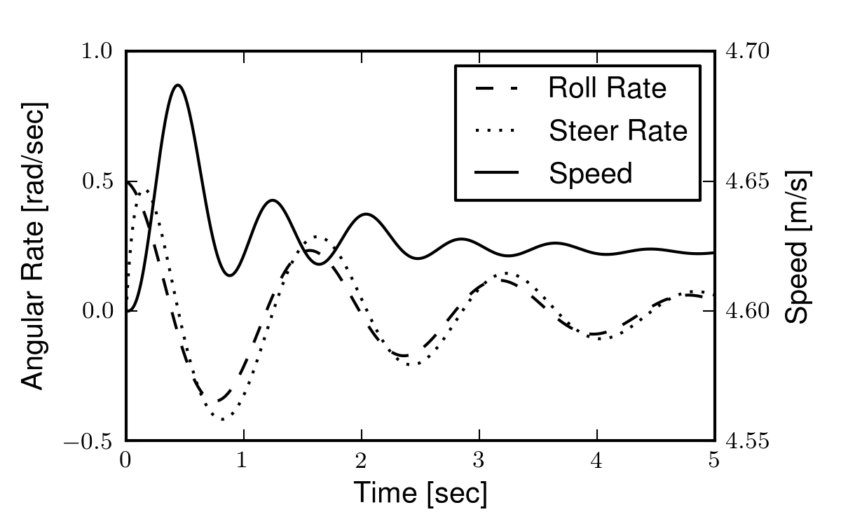
A reproduction of Figure 4 from [MPRS07]. For these initial conditions the model demonstrates stability. It also shows the energy conserving nature of the non-linear model (i.e. the forward speed settles to a higher value than the initial speed as the energy associated with lateral motion is transferred to the forward speed). Generated by src/eom/nonlinear_simulation.py.
Non-linear Validation
It is often difficult to validate that two independently derived multibody dynamical systems are equivalent. This due to mostly to the complexity of large analytical expressions which can be derived by different methodologies. A common method of validation is to evaluate the symbolic equations numerically for non-trivial inputs and compare the results to high precision. These type of numerical benchmarks are invaluable. They provide a baseline for model comparison allowing for scientific reproducibility and error checking.
[BMCP07] present the non-linear Whipple model derived with both the Newton-Euler and Lagrange methods, along with a numerical benchmark. Table 1 in their paper gives the derivatives of all the coordinates and speeds to high precision for both of their derivations at a single state. They claim that if one can compute the values to machine precision to ~10 significant figures then the models can be concluded to be the same[8].
The Basu-Mandal et al. derivations are based on different coordinates than those used here, but regardless of the coordinates they provide numerical values which can be benchmarked if the correct coordinate transformations are applied[9]. In Table 3.1[11] I present the values computed from the present model in comparison to the values presented in [BMCP07]. I’ve presented the same number of significant digits as provided by Basu-Mandall for each variable[10]. My model produces the same result to at least eleven significant figures, thus verifying the derivation is correct.
| Variable | Basu-Mandal | Moore |
|---|---|---|
| \(\beta_f\) | 0 | 0 |
| \(\dot{\beta_f}\) | 8.0133620584155 | 8.0133620584154 |
| \(\ddot{\beta_f}\) | 2.454807290455 | 2.454807290455 |
| \(\beta_r\) | 0 | 0 |
| \(\dot{\beta_r}\) | 8.912989661489 | 8.912989661489 |
| \(\ddot{\beta_r}\) | 1.8472554144217 | 1.8472554144220 |
| \(\phi\) | 3.1257073014894 | 3.1257073014894 |
| \(\dot{\phi}\) | -1.19185528069e-02 | -1.19185528069e-02 |
| \(\ddot{\phi}\) | 1.205543897884e-01 | 1.205543897886e-01 |
| \(\psi\) | 9.501292851472e-01 | 9.501292851472e-01 |
| \(\dot{\psi}\) | 6.068425835418e-01 | 6.068425835418e-01 |
| \(\ddot{\psi}\) | -7.8555281128244 | -7.8555281128245 |
| \(\psi_f\) | 2.311385135743e-01 | 2.311385135743e-01 |
| \(\dot{\psi_f}\) | 4.859824687093e-01 | 4.859824687093e-01 |
| \(\ddot{\psi_f}\) | -4.6198904039403 | -4.6198904039394 |
| \(\theta\) | 0 | 0 |
| \(\dot{\theta}\) | 7.830033527065e-01 | 7.830033527065e-01 |
| \(\ddot{\theta}\) | 8.353281706379e-01 | 8.353281706377e-01 |
| \(x\) | 0 | 0 |
| \(\dot{x}\) | -2.8069345714545 | -2.8069345714545 |
| \(\ddot{x}\) | -5.041626315047e-01 | -5.041626315048e-01 |
| \(y\) | 0 | 0 |
| \(\dot{y}\) | -1.480982396001e-01 | -1.480982396001e-01 |
| \(\ddot{y}\) | -3.449706619454e-01 | -3.449706619455e-01 |
| \(z\) | 2.440472102925e-01 | 2.440472102925e-01 |
| \(\dot{z}\) | 1.058778746261e-01 | 1.058778746261e-01 |
| \(\ddot{z}\) | -1.460452833298 | -1.460452833298 |
Linearized Equations of Motion
The non-linear equations of motion can be linearized about various equilibrium points. The obvious one is about the nominal configuration [MPRS07] but there are are an infinity of other associated with steady turns [BMCP07]. The equations can be linearized by computing the Taylor series expansion of the non-linear equations of motion about the equilibrium point of interest and disregarding the terms higher than first order. For the nominal configuration, this amounts to calculating the Jacobian of the system of equations with respect to the coordinates, speeds, and inputs to obtain the state matrix, \(\mathbf{A}\), and the input matrix, \(\mathbf{B}\). Output, \(\mathbf{C}\), and feed-forward, \(\mathbf{D}\), matrices are computed in the same fashion from the non-linear equations of the desired outputs. The partial derivatives of each equation were evaluated at the following fixed point: \(q_i=0\) where \(i=4,5,7\), \(u_i=0\) where \(i=4,7\), and \(u_5=-v/r_R\) where \(v\) is the magnitude of the component of velocity of the rear wheel center in the direction of travel. Care has to be taken when linearizing as \(q_5\) is a dependent coordinate which still appears on the right hand side of the equations. In general, the chain rule applies, but for the nominal configuration, the terms due to the implicit definition of pitch equal zero. The linearization transforms the system into four linear first order differential equations in the form
I calculate the equations symbolically to reach the same results presented in [MPRS07], but my equations are much lengthier because the simplification routines available in Autolev and SymPy where not that effective. [MPRS07] assumes linearity in their derivation from the start of the derivation and avoids many of the simplification issues. The accuracy of the linearized model was checked by comparing the numerical results to the benchmark bicycle in two ways. First the linearized equations of motion, Equation (55), were rearranged into two second order differential equations in the canonical form (Equation (56)) presented in [MPRS07]. They present the values for the coefficient matrices (\(\mathbf{M}\), \(\mathbf{C}_1\), \(\mathbf{K}_0\) and \(\mathbf{K}_2\)) for the benchmark parameter set to at least 13 significant figures and the linearization presented here matched all of the significant figures. [MPRS07] also provide the eigenvalues of the state matrix at various speeds. Table 3.2[12] shows the eigenvalues computed at 5 m/s compared to the values in Table 2 of [MPRS07]. These match to at least 13 significant figures.
| Model | Caster | Weave Real | Capsize | Weave Imaginary |
|---|---|---|---|---|
| Meijaard | -1.407838969279822e+01 | -7.7534188219585e-01 | -3.2286642900409e-01 | 4.46486771378823e+00 |
| Moore | -1.407838969279825e+01 | -7.7534188219584e-01 | -3.2286642900409e-01 | 4.46486771378822e+00 |
The lateral dynamics of this linear model are remarkably similar to the non-linear model especially around the regime of a typical bicycle’s operating point. Figure 3.5 gives an example simulation with the same initial conditions as the Figure 3.4. Notice that the lateral dynamics, steer and roll, are almost identical, but that the constant forward speed equilibrium condition destroys the conservative property demonstrated in the non-linear model.
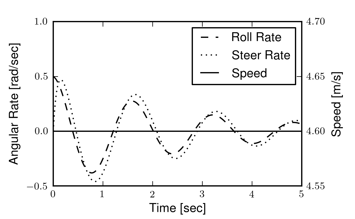
Simulation of the linear model given the same initial conditions as Figure 3.4. Generated by src/eom/linear_comparison.py.
It turns out that speed has profound effect on the lateral dynamics of the bicycle. It is useful to plot the root locus, Figure 3.6, of the characteristic equation with respect to the change in the equilibrium forward speed to visualize the time constants, damping, frequency, and stability of each of the modes of motion. The modes can be clearly identified along with the speed dependent stability.
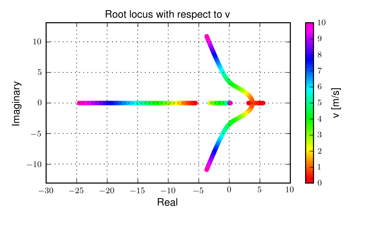
The root locus with respect to forward speed. The color variation signifies speed as shown in the right side color bar. Two eigenvalues are real, one being stable but increasingly fast and the other slowing to a marginally unstable location at high speed. The other two are initially real and unstable, but these coalesce into a complex pair and eventually become stable, at a higher moderately well damped frequency. Generated by src/eom/linear_comparison.py.
Another useful and popular way to visualize the root locus is by plotting the real and imaginary eigenvalue components separately versus forward speed, Figure 3.7. This view gives a clearer view of the stable speed range.
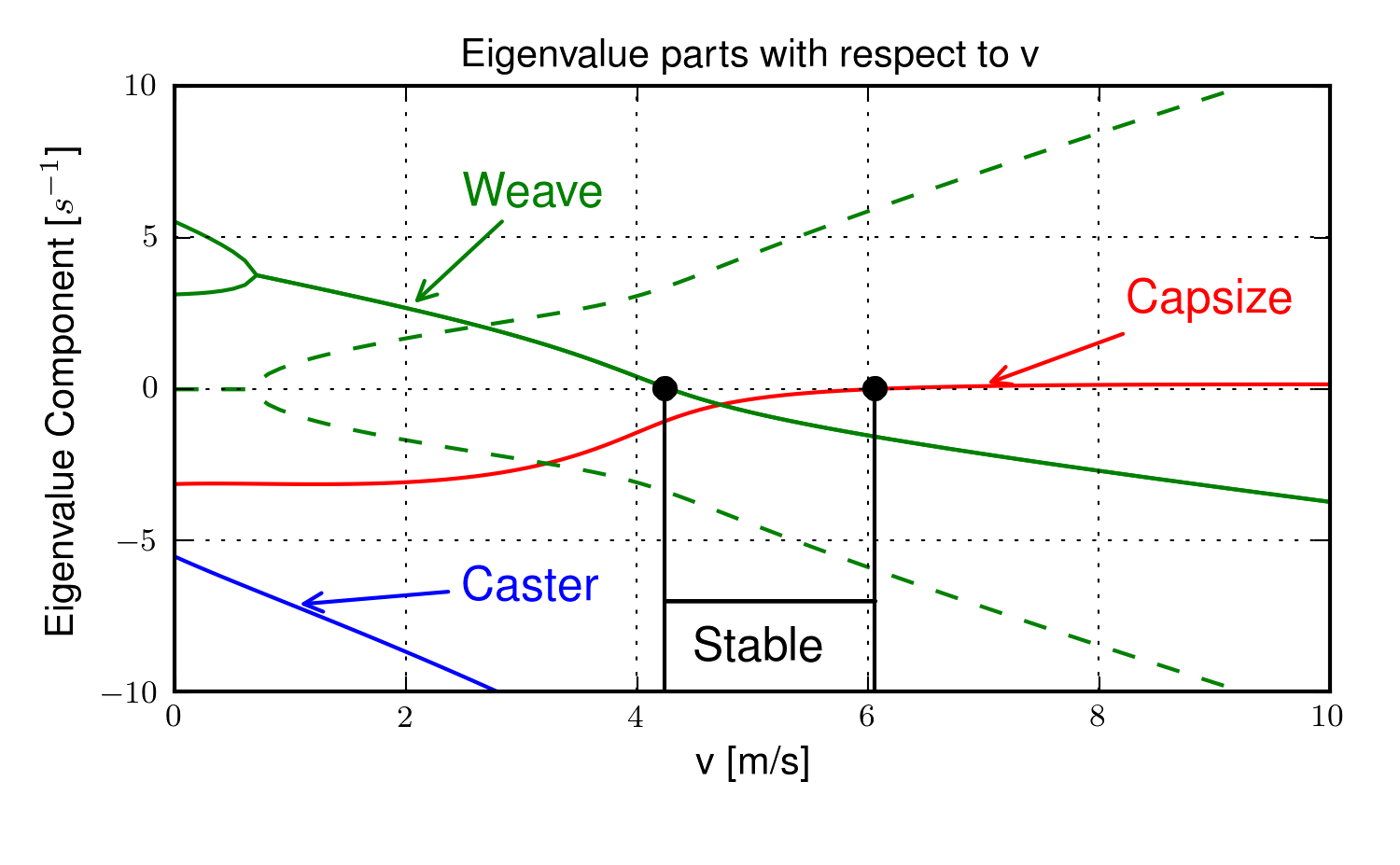
The real (solid) and imaginary (dashed) eigenvalue components versus speed for an example parameter set. The four modes of motion are identified. Caster is stable and real for all positive values of speed. It describes the tendency for the front wheel to right itself in forward motion. Capsize is always real and stable at low speeds but becomes marginally unstable at a higher speed. It describes the roll of the rear frame. Weave is real at very low speeds and describes an inverted pendulum-like motion i.e. the bicycle falls over. As speed increases the eigenvalues coalesce into a complex conjugate pair at the weave bifurcation that describes an exponentially increasing sinusoidal motion of roll and steer, with steer lagging the roll. This mode becomes stable at a higher speed. The weave and capsize critical speeds bound the stable speed range. Generated by src/eom/linear_comparison.py.
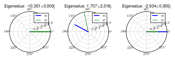
The behavior of the modes of motion can be visualized by plotting the eigenvector components in the complex plane for various speeds. For the speeds shown in the root locus plots, there are four distinct speed ranges of interest: below the weave bifurcation, between the weave bifurcation and the weave critical speed, the stable speed range, and above the capsize critical speed. At a forward speed of 0.5 m/s, all eigenvalues are real, with two unstable and two stable. In Figure 3.8, notice that the unstable eigenvalues predict two modes where the roll and steer states exponentially increase and with roll and steer 180 degrees out of phase. These modes describes a simple unstable inverted pendulum motion.
Normalized eigenvector components plotted in the real/imaginary plane for each mode at 5.0 m/s. Only the roll angle, \(q_4\), and steer angle, \(q_7\), components are shown. Generated by src/eom/plot_eigenvectors.py.
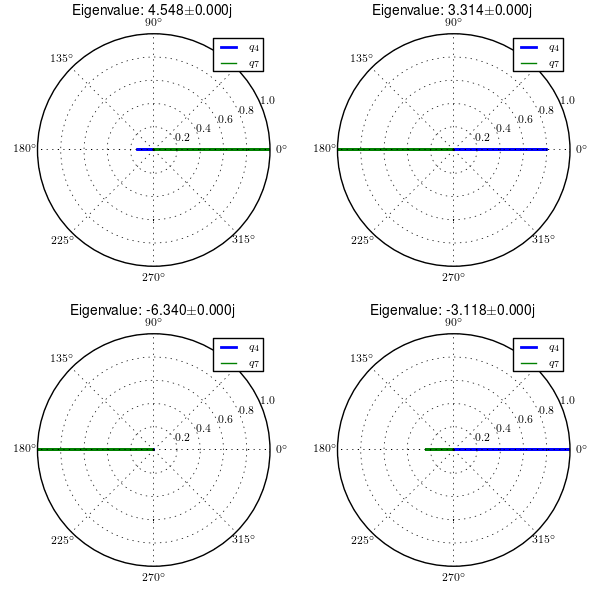
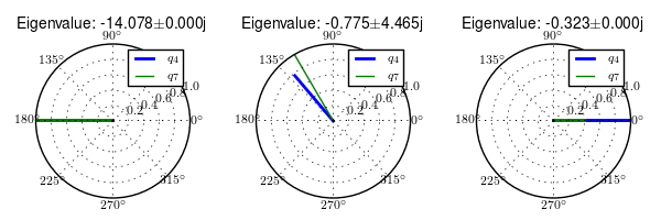
For speeds above the weave bifurcation speed, this linear model exhibits three distinct modes of motion, which have been named weave, capsize, and caster. As the bicycle is brought up to a speed of 3 m/s the two unstable eigenvalues coalesce into a complex pair. In Figure 3.9, the left-most graph depicts the caster mode which simply shows a rapidly decaying steer angle. The unstable weave mode eigenvector components show that the steer amplitude is about 25% larger than the roll amplitude and roll angle leads the steer angle by about 50 degrees. Finally, the capsize mode is a decays in roll and steer, with the roll at about twice the amplitude as steer.
Normalized eigenvector components plotted in the real/imaginary plane for each mode at 3.0 m/s. Only the roll angle, \(q_4\), and steer angle, \(q_7\), components are shown. Generated by src/eom/plot_eigenvectors.py
At 5 m/s all modes are stable with the weave mode showing that the roll now only leads the steer by about 10 degrees. The caster and capsize are similar to 3 m/s.
Normalized eigenvector components plotted in the real/imaginary plane for each mode at 5.0 m/s. Only the roll angle, \(q_4\), and steer angle, \(q_7\), components are shown. Generated by src/eom/plot_eigenvectors.py
Finally, at 7 m/s the capsize mode becomes unstable, with a slow exponential increase primarily in roll.
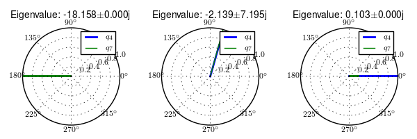
Normalized eigenvector components plotted in the real/imaginary plane for each mode at 7.0 m/s. Only the roll angle, \(q_4\), and steer angle, \(q_7\), components are shown. Generated by src/eom/plot_eigenvectors.py
The eigenvalues and eigenvectors describe the complete motion of the linear bicycle model where the motion from each mode is sum to gather the whole motion at a given speed. Typical diamond frame bicycle designs with an average sized rigid rider exhibit this basic behavior, but even small variations in some of the parameters can change the system behavior drastically, especially with regards to stability.
Parameter Conversion
This section details the conversion from the benchmark parameter set in [MPRS07] to the presented parameter set, Figure 3.2. As mentioned earlier, the Meijaard parameters are not a good choice when working with the non-linear derivation because most are not constant with respect to configuration. So the parameters must be converted to a configuration independent set. When the bicycle is in the nominal configuration the parameters can be converted with the following relationships.
Starting with the geometry, the wheel radii are defined the same, but the remaining geometry is calculated as
The mass center locations are
The masses are equivalently defined. Here the left side gives the present variables and the right gives the benchmark variables.
The moments of inertia of the wheels are also equivalently defined.
The moments and products of inertia for the frame and fork require the direction cosine matrix with respect to rotation through the steer axis tilt, \(\lambda\).
Notation
- \(A,B,C,D,E,F\)
- Reference frames and/or rigid bodies.
- \(d_1,d_2,d_3\)
- Distances that describe the rear and front frame essential geometry.
- \(l_1,l_2,l_3,l_4\)
- In plane distances to the rear and front frame centers of mass.
- \(m_C,m_D,m_E,m_F\)
- Mass of each rigid body.
- \(\mathbf{I}_C,\mathbf{I}_D,\mathbf{I}_E,\mathbf{I}_F\)
- Local inertia tensor of each rigid body.
- \(^Y\mathbf{R}^X\)
- Rotation matrix of body or reference frame \(X\) with respect to body or reference frame \(Y\).
- \(q_i\)
- Generalized coordinates.
- \(u_i\)
- Generalized speeds.
- \(\hat{x}_1,\hat{x}_2,\hat{x}_3\)
- Three orthogonal unit vectors in reference frame \(X\).
- \(x_o\)
- Mass center of body \(X\).
- \(c_e\)
- Point on the steer axis in both bodies \(C\) and \(E\).
- \(d_n,f_n\)
- Points fixed in the rear and front wheels which are instantaneously in contact with the ground.
- \(\bar{r}^{y_o/x_o}\)
- Vector from point \(x_o\) to point \(y_o\).
- \(^X\bar{\omega}^Y\)
- Angular velocity of frame \(Y\) in frame \(X\).
- \(^Y\bar{v}^{x_o}\)
- Velocity of point \(x_o\) in reference frame \(Y\).
- \(^X\bar{\alpha}^Y\)
- Angular acceleration of frame \(Y\) in frame \(X\).
- \(^Y\bar{a}^{x_o}\)
- Acceleration of point \(x_o\) in reference frame \(Y\).
- \(s_1,c_1\)
- Shorthand notation for \(\operatorname{sin}q_1\) and \(\operatorname{cos}q_1\).
- \(s_\lambda,c_\lambda\)
- Shorthand notation for \(\operatorname{sin}\lambda\) and \(\operatorname{cos}\lambda\).
- \(\tilde{F}_r\)
- Nonholonomic generalized active forces. The subscript \(r\) denotes one of the independent generalized speeds.
- \(^N\bar{V}_r^{x_o}\)
- rth partial velocity of point \(x_o\) in reference frame \(N\) with respect to the independent generalized speed, \(u_r\).
- \(\bar{R}^{x_o}\)
- Resultant forces on the point \(x_o\).
- \(^N\bar{\omega}_r^C\)
- rth partial angular velocity of reference frame \(C\) in reference frame \(N\) with respect to the independent generalized speed, \(u_r\).
- \(\bar{T}^C\)
- Resultant torques acting on body \(C\).
- \(\tilde{F}^*_r\)
- Nonholonomic generalized inertia forces. The subscript \(r\) denotes one of the independent generalized speeds.
- \(\bar{R}^*_{x_o}\)
- Generalized inertia force of point \(x_o\).
- \(\bar{T}^*_X\)
- Generalized inertia torque of body \(X\).
- \(I_X\)
- Central inertia dyadic of body \(X\).
- \(\mathbf{A},\mathbf{B},\mathbf{C},\mathbf{D}\)
- The state, input, output and feed-forward matrices.
The following benchmark parameters are all defined in [MPRS07].
- \(\lambda\)
- Steer axis tilt.
- \(c\)
- Trail.
- \(w\)
- Wheelbase.
- \(r_F,r_R\)
- Front and rear wheel radii.
- \(x_B,z_B,x_H,z_H\)
- Mass center locations of the rear frame and front frame.
- \(B,R,H,F\)
- Rigid bodies as defined in.
- \(m_B,m_R,m_H,m_F\)
- Mass of each rigid body.
- \(\mathbf{I}_B,\mathbf{I}_R,\mathbf{I}_H,\mathbf{I}_F\)
- Inertia tensor of each rigid body.
- \(v\)
- Forward speed of the linear bicycle model.
- \(\mathbf{M},\mathbf{C}_1,\mathbf{K}_0,\mathbf{K}_2\)
- Velocity and gravity independent mass, damping, and stiffness matrices of the linearized Whipple model.
- \(\bar{q}\)
- Essential coordinates.
Footnotes
| [1] | These programming growing pangs were especially harsh with Autolev. The program is unfortunately missing virtually all of the useful tools and paradigms found in full-featured programming languages. |
| [2] | Kane himself has done work on bicycle and motorcycle models and made use of his method to derive the equations of motion [Kan75], [Kan77a], [Kan77b], [Kan78], [MK79]. Furthermore, [VZ75] derived linear equations of motion of the bicycle and models developed with AutoSim also employ Kane’s method [Say90], [SLG99]. |
| [3] | Luke and I have dreamed of developing an open source version of Autolev for years and that has finally culminated through primarily Luke and Gilbert Gede’s efforts in the creation of sympy.physics.mechanics. |
| [4] | The coordinates are also used by [FSR90], among others. |
| [5] | I don’t necessarily agree that this is a great standard to follow, because it creates much unessary confusion when defining and mapping between parameterizations. The three axis pointing upward would be less error prone because a bicycle is never below the ground plane, except maybe in an academic. |
| [6] | The bicycle wheels’ points of contact are abstract points in dynamics. At any instant there are two coincident points at the contact location: one on the wheel and one on the ground. If no-slip rolling is assumed, both of these points are motionless, i.e. their velocities are zero. These points are distinctly different from the points that trace out the path on the ground of the wheel contact locations through time. Those points are not motionless and therefore do have a velocity. |
| [7] | This constraint can readily be modified to accomodate a non-flat ground. |
| [8] | The very first model I developed in 2006 would not have held up to this test. I owe the validity of my model to my lab mate, Luke, as his persistence and interest in minute detail helped me bring my model up to par. Several issues plagued both of our derivations. The first was an simple missing apostrophe in my Autolev code, the second was that we had defined our rear wheel rotation with respec to the \(B\) frame instead of the \(C\) frame, the third was incorrect parameter conversions from the [MPRS07] paper to our parameters, and the fourth was a bug in my original code that I never found, with an entire code rewrite finally giving me matching eigenvalues. |
| [9] | The conversion equations from the [BMCP07] coordinates to the present set and vice versa can be found in the source code for the DynamicistToolKit bicycle module. |
| [10] | Basu-Mandall presents varying significant digits from 10 to 14. |
| [11] | The variable names correspond to the convention provided in [BMCP07]. This table is generated with src/eom/basu_comparison.py. |
| [12] | This table is generated with src/eom/linear_comparison.py. |
