Extensions of the Whipple Model
Preface
After I had derived the Whipple model, it was natural to start thinking about extending it to understand various other phenomena. It turned out that one of Mont’s former students, David de Lorenzo, had worked on adding rider biomechanical degrees of freedom to the Whipple model in the early 90’s, submitted the work to Vehicle System Dynamics but never resubmitted after the first round of reviews, and the work was still sitting dormant in Mont’s files. Luke and I had just finished our preliminary exams and decided to try to write a paper for the 2007 International Symposium on Computer Simulation in Biomechanics. de Lorenzo’s work inspired us to explore a model with more realistic rider motion, which we based on this dormant model. This was the first of several model extensions I developed for various reasons over the years. Others included variations on the rider biomechanics and models of unusual bicycle products such as the Swing Bike and Gyro Bike. This chapter details the findings from some of the models.
Introduction
The Whipple model is an ideal basic model and platform from which to explore more realistic models of both the bicycle and the rider. It has been demonstrated that the linear Whipple model can reliably predict the motion of a riderless uncontrolled bicycle [Koo06], [KSM08], [KS09], [Ste09], [ER11] for speeds in and around the stable speed range. But the Whipple model may certainly be limited in it’s ability to predict the motion of the bicycle and rider as an integrated system. A person’s body keeps its shape through passive joint forces, unconscious active control and conscious active control. Assuming no active control and lumping the unconscious control with the passive control one can potentially model the rider as flexible assembly of many bodies. Secondly, the rider’s weight is typically 80 to 90 percent of the entire system, which potentially invalidates the knife edge wheel assumptions employed in the Whipple model. Here I present several bicycle models that attempt to explain some of the rider’s passive dynamics and also a model with a passive stability augmentation device. The models are all based on the basic formulation of the Whipple model in Chapter Bicycle Equations Of Motion and make use of the variables defined therein. Various combinations of these model extensions are used in the later Chapters for analysis of more complicated systems.
Notation
Each model presented in this chapter makes use of the notation defined in Chapter Bicycle Equations Of Motion otherwise each model in each section is treated independently and may use the same notation of the other models.
Lateral Force Input
The Whipple model is typically defined with three inputs: roll torque \(T_4\), rear wheel torque \(T_6\), and steer torque \(T_7\). These ideal inputs are not necessarily easy to map to the actual inputs to the system. In particular, it is generally not possible to execute a pure roll torque, but a lateral force from the environment is much easier. This type of input has long been used and modeled, e.g. [Rol73] uses a lateral perturbation in modeling and experimentation of a motorcycle.
Here I add a fourth input, a lateral force \(F_{c_l}\), which acts at a point on the rear frame, \(c_l\). The force is defined such that it is always in the \(\hat{n}_2\) direction and acts on the point located in the mid-plane of the bicycle frame. The \(\hat{n}_2\) direction is chosen instead of the yaw frame’s \(\hat{a}_2\) direction because it better models the impulsive forces applied in the experiments detailed in Chapter System Identification. The force can describe a person walking beside a bicycle and simply pushing laterally on the rear frame. One can even think of it as a simplified version of the resultant force from lateral wind gust, although a gust would also apply a force to the front frame.
The vector from the rear wheel center to the lateral force point is
The velocity of the point is
where
To form the equations of motion, an additional generalized active force dot multiplied with the partial velocities of the point is required. The generalized active force is simply
The non-linear and linear models are computed in the same fashion as described in Chapter Bicycle Equations Of Motion, with an additional column in both the input, \(\mathbf{B}\), and feed-forward, \(\mathbf{D}\), matrices corresponding to the new input force. Unlike a pure roll torque this force can effectively contribute to both the roll and steer torques. The location of the point determines the contribution.
Figure 4.1 compares the impulse response for roll torque to that of a lateral force at the seat for a particular bicycle within its stable speed range. Notice that the lateral force input does not excite the system with as large amplitudes but that the response is similar. The amplitude is a function of where the force is applied. If the force is applied directly above the rear wheel contact at a height of unity from the ground, the response will be identical.
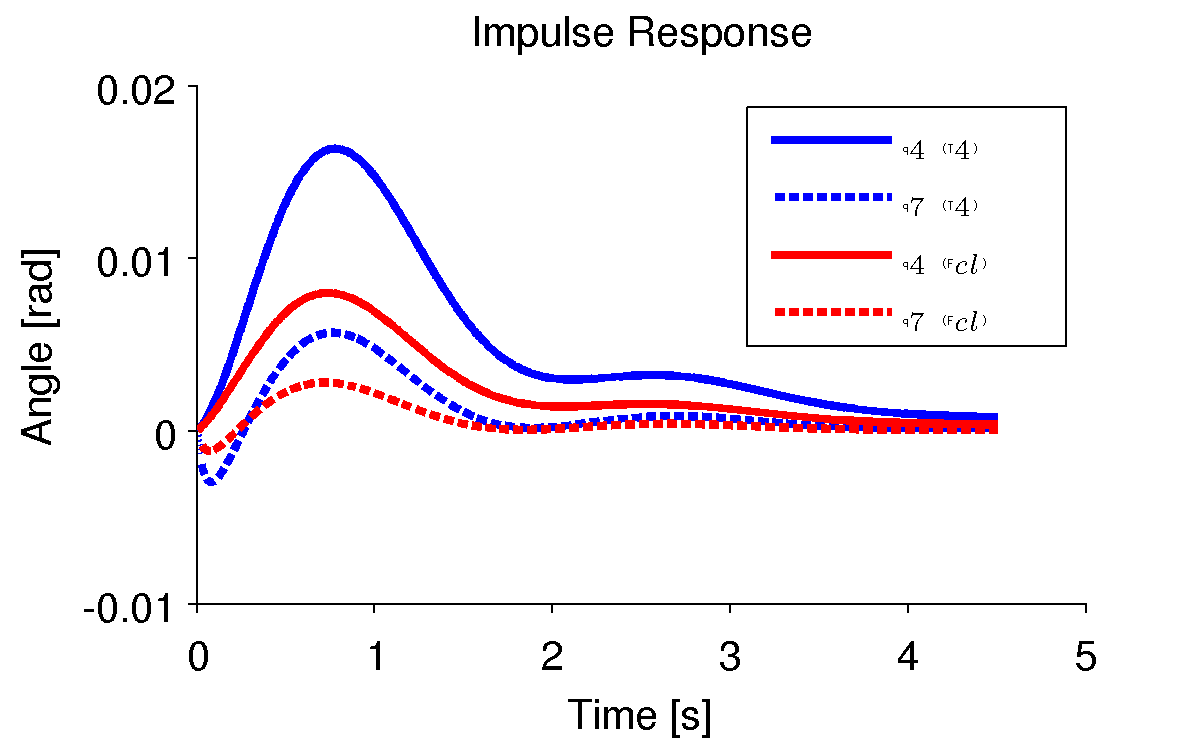
Impulse responses for the roll angle, \(q_4\), and steer angle, \(q_7\), for a roll torque input (blue) and the lateral force input at a point just below the seat (red). The numerical parameters were generated from the data of Jason on the Davis instrumented bicycle and the equations were linearized at a forward speed of 7 m/s. Plot generated by src/extensions/lateral/lateral_force.m`.
Figure 4.2 shows the frequency response in a similar fashion as the impulse response. The responses for both input types are very similar for this frequency range, with the difference in magnitudes a function of the distance the lateral force is from the rear wheel contact point.
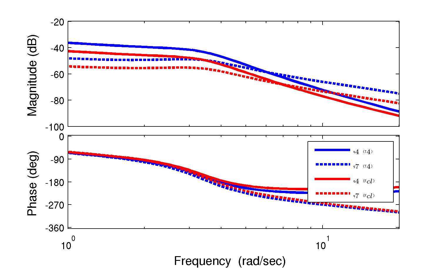
Frequency responses for the roll angle, \(q_4\), and steer angle, \(q_7\), for a roll torque input (blue) and the lateral force input at a point just below the seat (red). The numerical parameters were generated from the data of Jason on the Davis instrumented bicycle and the equations were linearized at a forward speed of 7 m/s. Plot generated by src/extensions/lateral/lateral_force.m.
This model is used extensively in the later chapters for modeling and simulation of lateral perturbation experiments.
Notation
- \(c_l\)
- The point at which the lateral force is applied.
- \(d_4,d_5\)
- The distances which locate the lateral force point \(c_l\).
- \(F_{cl}\)
- The magnitude of the lateral force.
Rider Arms
[SK10b] and [SMK12] has shown that the addition of the inertial effects of the arms can significantly alter the open loop dynamics of the bicycle-rider system, and most importantly, that a typical bicycle and rider may not have a stable speed range. As will be described in Chapter Davis Instrumented Bicycle, we rigidified the rider’s torso and legs with respect to the rear frame of the bicycle. The rider was then only able to make use of their arms to control the bicycle. The Whipple model does not take into account the dynamic motion of the arms and certainly not the fact that steer torques are actually generated from the muscle contraction and flexion in the riders arms. Being that our riders were able to move their arms and the motion can have significant effect on the open loop dynamics, we developed a similar model as the upright flexed arm model found in [SK10b] and [SMK12].
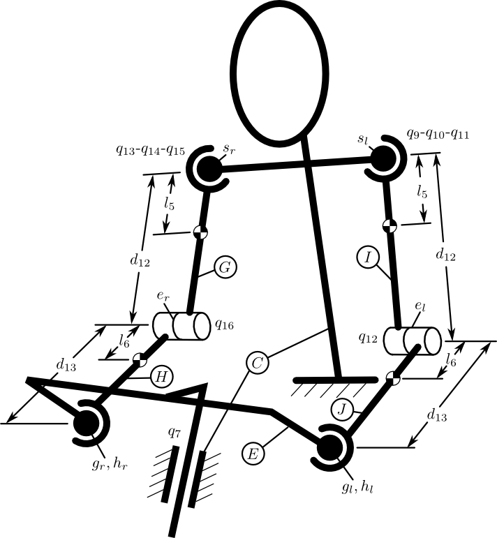
Diagram of the additional arm bodies. Only the upper portion of the system is shown. The rider’s torso, neck, and head are assumed to be part of the rear frame rigid body, \(C\).
In most bicycle models, the front frame is externally forced to move with respect to the rear frame through a torque applied between the rear frame and the front frame. A more realistic model with arms would force the front frame motion through joint torques in the arms. For simplicity’s sake and without loss of generality we keep the steer torque, \(T_4\), as the driving torque but retain the associated motion of the arms. The inertial effects of the arms can then be captured by adding four additional rigid bodies to the Whipple model for the left and right upper and lower arm segments and introducing enough constraints such that the additional degrees of freedom are removed Figure 4.3. The arms are assumed to symmetric with respect to the sagittal plane when in the nominal configuration. The four new bodies are defined as:
- \(G\):
- right upper arm
- \(H\):
- right lower arm
- \(I\):
- left upper arm
- \(J\):
- left lower arm
The right and left upper arms are each oriented through body fixed 1-2-3 rotations through the abduction, elevation and rotation angles \(q_9\), \(q_{10}\), \(q_{11}\) and \(q_{13}\), \(q_{14}\), \(q_{15}\) for the right and left arms respectively.
The right and left lower arms are oriented through simple rotations through \(q_{12}\) and \(q_{16}\) with respect to the upper arms at the elbow joint.
This definition differs from [SK10b] and will allow full non-linear unlocked motion of the arms. Schwab’s joint configuration limits the model to be valid only in and around the linear equilibrium point presented therein.
The right and left shoulders are located in the rear frame by
The right and left elbows are located by
The upper and lower arm mass centers are located by
The hands are located by
The handlebar grips are located by
To enforce that the hands remain on the grips, I first introduce six holonomic constraints embodied in
After forcing the hands to be at the grips this leaves two degrees of freedom, one for each arm. The free motion is such that the arms can rotate about the lines connecting the shoulders to the grips. I choose to eliminate these two degrees of freedom by forcing the arms to always “hang down” relative to the rear frame, i.e. that the vector aligned with the elbow has no component in the downward direction of the roll frame, \(B\).
This assumption is limited in validity to small pitch angles, as a large pitch angles would cause the riders arms to rotate in odd positions. A better constraint would be to dot with a vector in the \(C\) frame which is aligned with \(\hat{b}_3\) when the bicycle is not pitched, but this definition would require a new geometric parameter so I chose the former, i.e. Equation (13).
With these eight holonomic constraints, the model now has three degrees of freedom which are the same number as the Whipple model, but with the added inertial effects of the arms. The expressions for the velocities and accelerations of the mass centers of the four new bodies needed to form the equations of motion are lengthy and they are omitted here. Please refer to the source code for the equations: src/extensions/arms/Arms.al.
The generalized active forces remain the same as described in Chapter Bicycle Equations Of Motion with the addition of the lateral force described in the previous section. The generalized inertia forces must be modified to include the accelerations of the mass centers along with the mass and inertia of the new bodies. The masses are simply defined as \(m_g\), \(m_h\), \(m_i\) and \(m_j\). The arms segments are assumed to be symmetric about their associated \(3\) axes, thus \(I_{11} = I_{22}\).
With this information the equations of motion can be formed with Kane’s method as described in Chapter Bicycle Equations Of Motion. Special care must be taken when linearizing the equations of motion due to the eight holonomic constraints. The additional generalized coordinates, \(q_9\) through \(q_{16}\), are dependent coordinates and are ultimately functions of the pitch and steer angles. The chain rule must be properly applied or the independent coordinates must be solved for when expanding the Taylor series and forming the Jacobian matrices.
Figures 4.4 and 4.5 show how the eigenvalues vary with speed with respect to the nominal configuration equilibrium point. There are three distinct modes for all speeds shown, two of which are real and one that is complex. The oscillatory mode is always stable, unlike the weave mode in the Whipple model. Secondly, one real mode is always unstable and the other is always stable. The addition of the arms’ inertial effects causes the system to not have a stable speed range unlike the prediction of the Whipple model.
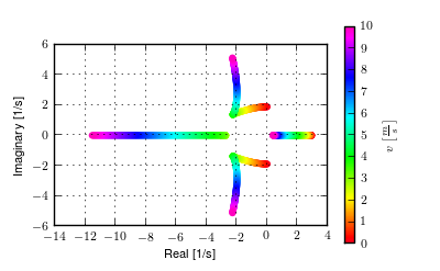
The root locus with respect to speed of the Whipple model with arms for the parameter set associated with Jason seated on the Davis instrumented bicycle calculated with the Yeadon method. Generated with src/extensions/arms/plot_eig.py.
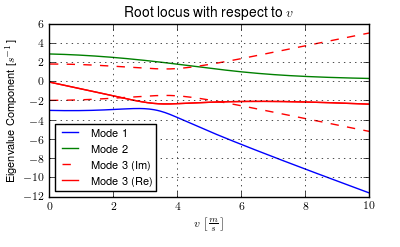
The components of the eigenvalues with respect to speed of the Whipple model with arms for the parameter set associated with Jason seated on the Davis instrumented bicycle calculated with the Yeadon method. This plot shares similar characteristics as the one presented in [SK10b]. Generated with src/extensions/arms/plot_eig.py.
One may be quick to parallel the three modes of motion to the weave, capsize, and caster modes of the Whipple model, but closer examination of the eigenvectors reveals that the motions are not quite the same. Figures 4.6, 4.7, 4.8, and 4.9 are phasor plots of the eigenvector components at various speeds which correspond to the ones given in previous chapter for the Whipple model.
The phasor diagrams show that the most negative real eigenmode is not as nearly as fast as the caster mode and it is no longer dominated by steer angle. The mode decays in both roll and steer with roll dominant at low speeds and steer at high speeds. The unstable real eigenmode is dominant in roll angle and slows with increasing speed like the Whipple model, but is unstable for the given speeds. The stable oscillatory mode is dominant in steer at low speeds and roll at high speeds. The 0.5 m/s case is interesting in that the mode is primarily a stable oscillation in steer angle around 0.3 hertz. As the speed increases the larger roll angle magnitude is different in behavior than the Whipple weave mode.
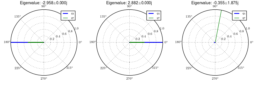
Normalized eigenvector components plotted in the real/imaginary plane for each mode at a forward speed of 0.5 m/s. Only the roll angle, \(q_4\), and steer angle, \(q_7\), components are shown. Generated with src/extensions/arms/plot_eig.py.
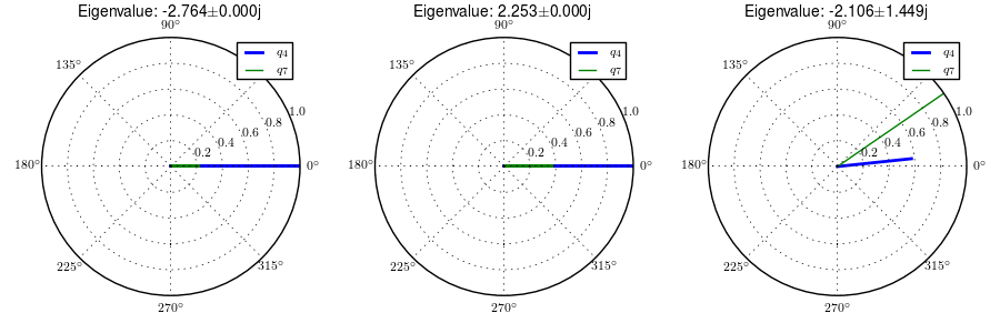
Normalized eigenvector components plotted in the real/imaginary plane for each mode at a forward speed of 3.0 m/s. Only the roll angle, \(q_4\), and steer angle, \(q_7\), components are shown. Generated with src/extensions/arms/plot_eig.py.
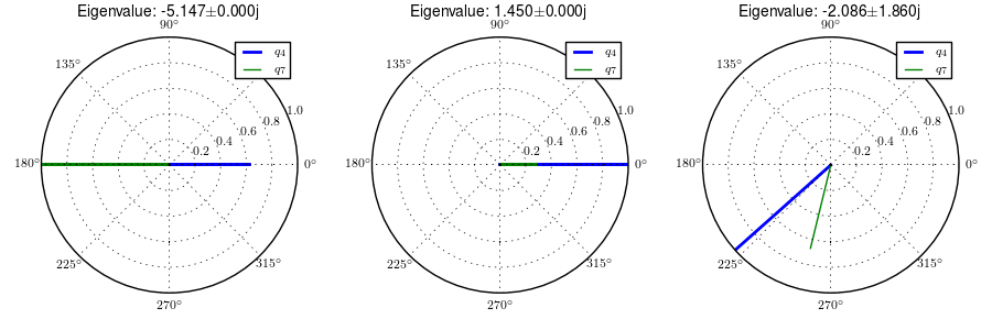
Normalized eigenvector components plotted in the real/imaginary plane for each mode at a forward speed of 5.0 m/s. Only the roll angle, \(q_4\), and steer angle, \(q_7\), components are shown. Generated with src/extensions/arms/plot_eig.py.
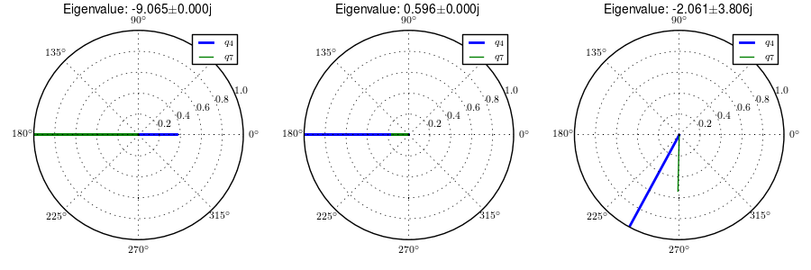
Normalized eigenvector components plotted in the real/imaginary plane for each mode at a forward speed of 8.0 m/s. Only the roll angle, \(q_4\), and steer angle, \(q_7\), components are shown. Generated with src/extensions/arms/plot_eig.py.
Notation
- \(G,J,I,J\)
- The arm rigid bodies.
- \(d_6\)-\(d_{13}\)
- Geometric distances to locate the arm joints.
- \(s_r,e_r,h_r,g_r,s_l,e_l,h_l,g_l\)
- Points on the arms and handlebars: (s)houlder, (e)lbow, (h)and, and (g)rip. Subscripts: (l)eft and (r)ight.
- \(m_g,m_h,m_i,m_j\)
- The masses of the arm rigid bodies.
- \(\mathbf{I}_G,\mathbf{I}_H,\mathbf{I}_I,\mathbf{I}_J\)
- The inertia tensors of the arm rigid bodies defined about the mass center and with respect to the local reference frame.
Front wheel flywheel
Another model extension of interest involves addition of an extra rotating wheel coincident with the front wheel. It is well known that that increasing the angular momentum of the front wheel via change in inertia ([ASKL05], [FSR90]) or rotational speed, has a strong effect on the stability of the Whipple model. For the benchmark bicycle [MPRS07], independently increasing the moment of inertia of the front wheel, decreases both the weave and capsize speeds. A low weave speed may provide open loop stability advantages to riders at low speed, with the reasoning that a stable bicycle may require less rider control. Conversely, it has also been shown both that a bicycle without gyroscopic effects can be stable [KMP+11] and that humans can ride them [Jon70] with little difficulty. The idea that gyroscopic action can stabilize a moving two wheeled vehicle has been demonstrated as early as the dawn of the 20th century, with the invention of the gyro monorail and the gyro car ([Wik12a], [Wik12b]) which made use of control servos to gyros to applied roll righting torques to the single track vehicles. Of more recent interest, several engineering students at Dartmouth University applied this theory to a compact flywheel mounted within the spokes of a children’s bicycle wheel [War06] taking advantage of the fact that the flywheel imparts torques such that the bicycle steers into the fall. This has since been developed into a commercially available product, the GyroBike, that claims to allow children to learn to ride more easily, due to the bicycle’s increased stability at low speeds. I was given an article about the bicycle from the Dartmouth alumni magazine, subsequently met the woman who created the startup company around the idea in San Francisco, was able to test ride the full scale prototype, and eventually purchased a 12” version of the bicycle. The bicycle alone stays very stable even to extremely low speeds, but when I, as an experienced rider, tried to ride and control it the steering felt less responsive than one would generally prefer.
The following video demonstrates that the gyrobike without a rider is stabilized at 2 m/s when the flywheel is at full speed.
Using the Whipple model presented in Chapter Bicycle Equations Of Motion as a base, the flywheel’s effect can be modeled by adding an additional symmetric rigid body, \(G\) with mass \(m_g\) to the system which rotates about the front wheel axis though a new generalized coordinate, \(q_9\). The angular velocity and acceleration of the new body are defined with the simple kinematical differential equation
where
The location of the flywheel center of mass is at the same point as the front wheel center of mass, making the linear velocities and accelerations the same as the front wheel
An additional torque, \(T_9\), is required to drive the flywheel relative to the front wheel
At this point, \(\tilde{F}_r\), can be formed with an additional equation for the new degree of freedom.
The generalized inertia force, \(\tilde{F}^*_r\) is formed by taking into account the mass, \(m_g\), and inertia of the new body
The equations of motion are formed and linearized with respect to the nominal equilibrium point and a nominal angular velocity of the flywheel. Figures 4.10, 4.11, 4.12, and 4.13 show how adjusting the flywheel angular velocity can affect the stability of the bicycle which may be beneficial for people learning to ride a bicycle. All of the plots were generated using parameters measured from a production GyroBike and the rider’s parameters were generated by scaling the Yeadon geometry of an adult, Charlie, to child-size proportions which are detailed in Chapter Physical Parameters.
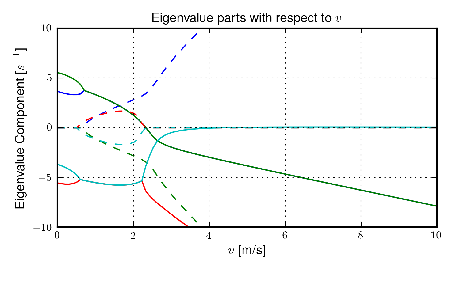
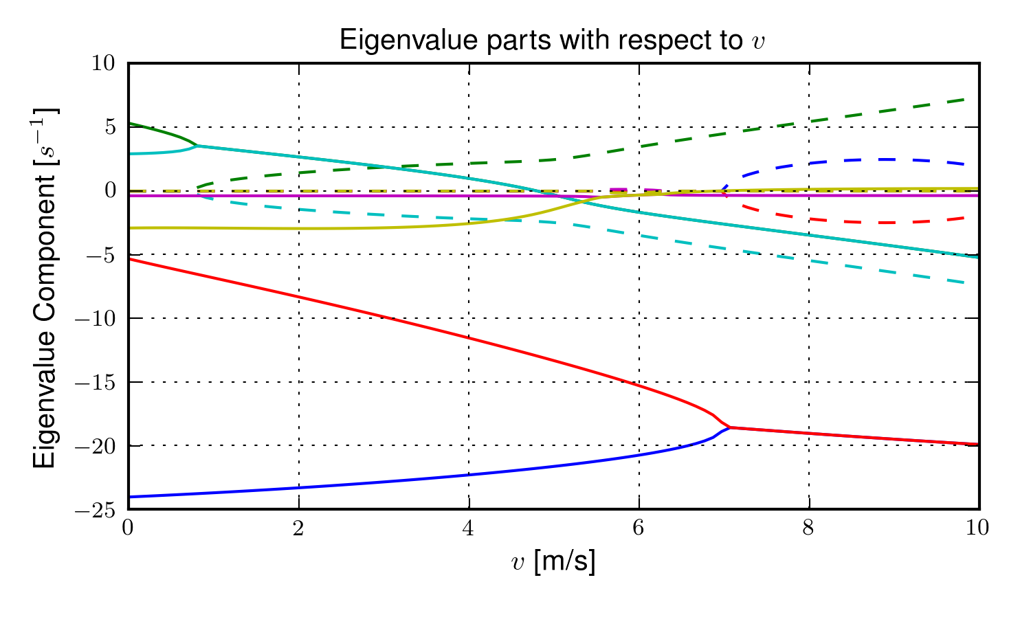
The magnitudes of the eigenvalue components with respect to the forward speed when the flywheel is fixed to the front wheel (i.e. has the same angular velocity as the front wheel). The solid lines show the real parts and the dotted lines show the imaginary parts, with color matching the parts for a given eigenvalue. Generated by src/extensions/gyro/gyrobike_linear.py.
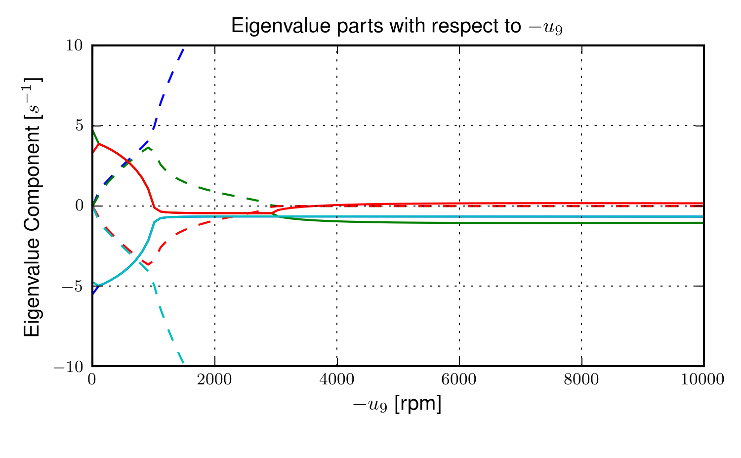
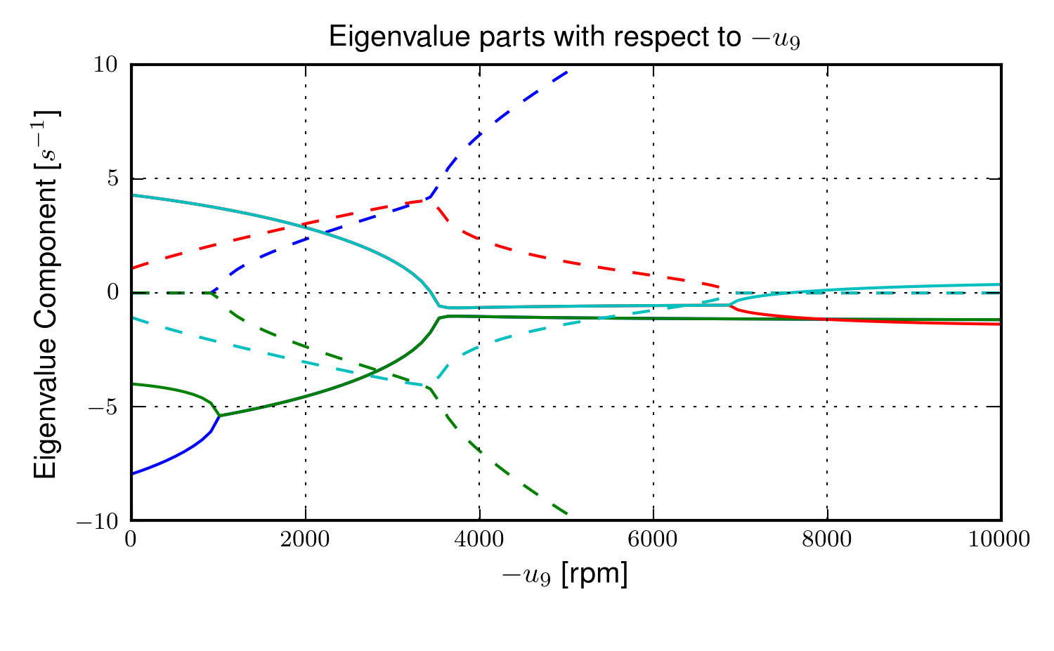
The magnitudes of the eigenvalue components with respect to the flywheel angular speed when the forward velocity is 0.5 m/s. The solid lines show the real parts and the dotted lines show the imaginary parts, with color matching the parts for a given eigenvalue. Generated by src/extensions/gyro/gyrobike_linear.py.
Figure 4.10 depicts similar dynamics as one would expect from a riderless bicycle with a relatively low weave critical speed (~2.25 m/s). Figure 4.11 then shows that the very unstable system at low speeds can certainly be made stable by increasing the angular velocity of the flywheel. In particular the bicycle becomes stable around 1000 rpm but it is also interesting to note that increasing the velocity too much (> 3500 rpm) results in an unstable system. The actual Gyrobike flywheel spins at speeds up to 2000 rpm and riderless stability can clearly be observed.
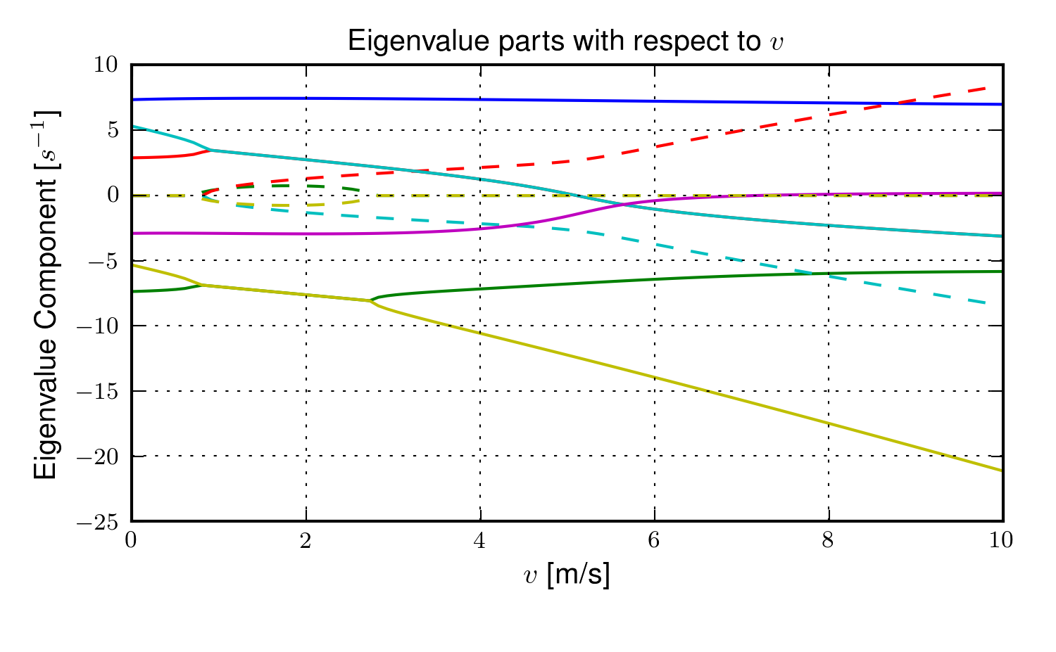
The magnitudes of the eigenvalue components with respect to the forward speed when the flywheel is fixed to the front wheel (i.e. has the same angular velocity as the front wheel) and a rigid child is seated on the bicycle. The solid lines show the real parts and the dotted lines show the imaginary parts, with color matching the parts for a given eigenvalue. Generated by src/extensions/gyro/gyrobike_linear.py.
The magnitudes of the eigenvalue components with respect to the flywheel angular speed when the forward velocity is 0.5 m/s and a rigid child is seated on the bicycle. The solid lines show the real parts and the dotted lines show the imaginary parts, with color matching the parts for a given eigenvalue. Generated by src/extensions/gyro/gyrobike_linear.py.
Figure 4.12 shows that the weave critical speed with a rider is only about 1 m/s greater than without a rider. Figure 4.13 shows that if a child-sized rider is rigidly added to the rear frame that the flywheel must spin up to 3500 rpm for the system to be stable and the time constant of the unstable eigenvalue does not decrease significantly until the flywheel spins at 2000 rpm. Also as with the riderless case, the system can be destabilized if the wheel spins at a high enough rate; in this case about 7000 rpm.
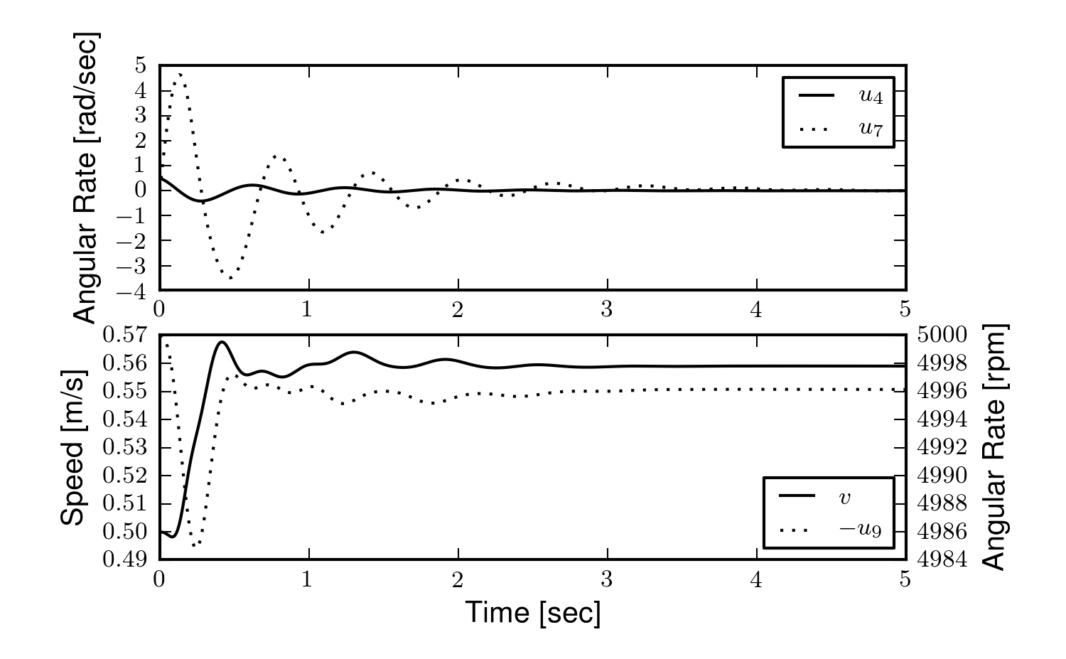
The open loop non-linear simulation of the gyro bicycle given the initial conditions: \(u_4=0.5\) rad/s, \(u_6=-v/r_R\) where \(v=0.5\) m/s, \(u_9=-5000\) rpm.
Figure 4.14 shows the resulting time history of the non-linear model traveling at a very slow speed with the flywheel spinning fast enough to stabilize the bicycle. The gyroscopic torques cause the steer angle to decay rapidly in a steer into the fall. The conservative nature of the system causes the forward speed to increase slightly. This is reflected as a decrease in the flywheel rotational speed because it is defined with respect to the front wheel.
This model and these examples give credence to the effectiveness of increasing the angular momentum of the front wheel in stabilizing the bicycle. The gyroscopic forces may not be necessary for stability but they have great power in stabilizing even very unstable systems. This assistance does come a cost though, both in the flywheel weight and the need to spin the flywheel at high speeds. When the child rider’s inertia is accounted for, very high spin speeds are needed to stabilize the system. And interestingly, increasing the flywheel speed too much can destabilize the system, albeit only marginally.
Notation
- \(G\)
- The flywheel rigid body.
- \(m_g\)
- Mass of the flywheel.
- \(q_9\)
- Angle of the flywheel with respect to the front wheel.
- \(u_9\)
- Angular rate of the flywheel with respect to the front wheel.
- \(g_o\)
- Flywheel mass center.
- \(T_9\)
- Torque acting between the front wheel and the flywheel.
- \(\mathbf{I}_G\)
- Inertia tensor of the flywheel.
- \(v\)
- The forward speed of the bicycle: \(v = - r_R u_6\).
Leaning rider extension
A common assumption regarding how a person biomechanically controls a bicycle with minimal or no input via the handlebars is that the rider can lean their body relative to the bicycle rear frame. This assumption is more often than not drawn from observing no-hands riding during which the rider seems to lean relative to the bicycle frame. A simple leaning rider can be modeled by adding an additional rider upper body as an inverted pendulum atop the bicycle. This introduces an additional lean degree of freedom, \(q_9\), and can be accompanied by a rider lean torque, \(T_9\) which models the rider’s ability to apply forces between the upper torso and the rear frame.
Many have created variations of this model in the past including [VLS67], [RL72], [Wei72], [VZ75], [Nag83], etc. but, as [RL72] points out, the roll torque is the more realistic control input as opposed to roll angle as many of the other authors tend to prefer. Weir et al. notes the fact that lean control has much less authority than steer control, and that the rider more or less leans equal and opposite to the vehicles roll angle [WZT79]. The inverted pendulum with a roll torque has now been widely adopted and more recent works focus on understanding these types of models ([Sha07a], [Sha08], [SKM08], [PH08b], etc.), with the hypothesis that control by roll torque is much less effective than steer torque being confirmed in all these studies.
To build the same model, we define the upper body hinge as a horizontal line at a distance \(d_4\) below the rear wheel center when the bicycle is in the nominal configuration. The direction cosine matrix relating the upper body to the rear frame is
A point, \(c_g\), on the hinge is then defined as
where \(\lambda\) is the steer axis tilt and is a function of \(d_1\), \(d_2\), and \(d_3\) as described in Bicycle Equations Of Motion.
The mass center is located by
The angular velocity and angular acceleration of the upper body in the bicycle frame is defined as
with \(u_9=\dot{q}_9\). The linear velocities of the hinge point and the upper body center of mass are
where
and
where
The linear accelerations of the hinge point and the upper body center of mass are as follows
where
and
and
where
where
We introduce two additional torques. The first is an input torque between the rear frame and the rider’s upper body, \(T_9\). This can be considered as the active torque contribution which the rider’s control system would provide. The second torque is defined as
where \(c_9\) and \(k_9\) are damping and stiffness coefficients which are provided as way to characterize the passive torques generated by the tissue, ligament, tendon, and bone structures. A free lean joint without this passive torque is far from realistic as large active torques would be required to keep the body upright. These are equivalent to simple proportional and derivative negative feedback on the roll angle and could be defined as such equivalently.
The additional generalized force is
and the generalized torques are modified to include the new torques
The mass of the upper body is \(m_g\) and it is assumed to by symmetric about its sagittal plane
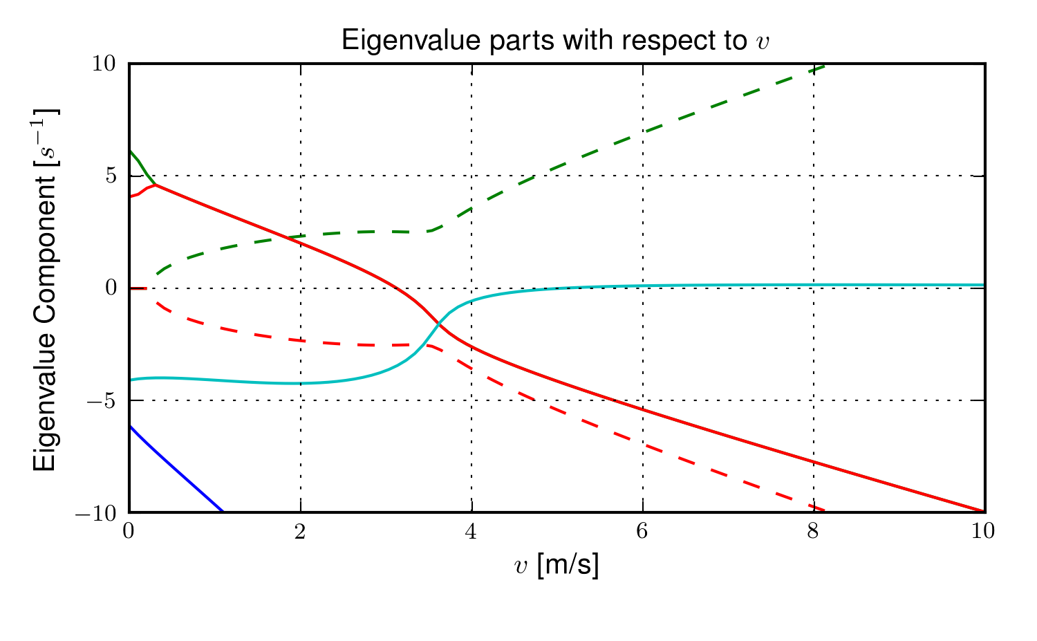
The equations of motion are again formed using Kane’s method and linearized as described in Chapter Bicycle Equations Of Motion. This linear model has been explicitly explored by both [SKM08] and [PH08b] with parameter values estimated by proportioning the benchmark parameter set from [MPRS07]. The following plot, Figure 4.15, uses more realistic rider parameters which are generated with methods described in Chapter Physical Parameters and the passive lean torque coefficients are set to zero to demonstrate the nature of the system with no passive stiffness and damping. Notice that the largest eigenvalue is much larger than those reported in Schwab and Peterson with a time to double of about a tenth of a second. We found that root difficult to stabilize when employing a manual control model based on the one presented in Chapter Control, which suggests the need and existence for some additional passive stabilization.
The magnitudes of the eigenvalue components with respect to the forward speed for the leaning rider model. The solid lines show the real parts and the dotted lines show the imaginary parts, with color matching the parts for a given eigenvalue. Generated by src/extensions/lean/riderlean.py.
The damping and stiffness coefficients can be selected such that the highly unstable rider mode is stabilized and the stable speed range observed in the Whipple model is restored, Figure 4.16. It is likely that control strategies that work with the Whipple model can be applied to this model with appropriate stiffness and damping selections. The parameters used are taken from [DLH96], which he estimated to be, \(k_9=128\) N-m/rad and \(c_9=50\) N-m/rad/s.
The magnitudes of the eigenvalue components with respect to the forward speed for the leaning rider model. The solid lines show the real parts and the dotted lines show the imaginary parts, with color matching the parts for a given eigenvalue. Generated by src/extensions/lean/riderlean.py.
The leaning rider model exhibits a very fast, unstable eigenmode which is constant with respect to speed when the upper body is treated as a simple inverted pendulum. In general, rider lean degrees of freedom have a de-stabilizing effect to the Whipple model. A combination of the rider’s active and passive postural control most likely stabilizes this mode in the real system, but it is debatable whether the passive control alone completely stabilizes the mode.
Notation
- \(d_4\)
- The distance to the torso hinge.
- \(l_5,l_6\)
- Distances to locate the upper body mass center.
- \(s_{\lambda-5}\), \(c_{\lambda-5}\)
- Shorthand for \(\operatorname{sin}(\lambda-q_5)\) and \(\operatorname{sin}(\lambda-q_5)\).
- \(c_g\)
- Rider hinge point.
- \(c_9,k_9\)
- The passive stiffness and damping coefficients.
- \(m_g\)
- Mass of the upper body (torso, arms, neck, and head).
- \(\mathbf{I}_g\)
- Inertia of the upper body.
- \(T_9\)
- The active torque acting between the rider’s upper body and the rear frame.
- \(T_9^p\)
- The passive torque acting between the rider’s upper body and the rear frame.
David de Lorenzo extension
Preface
To expand on the ideas presented in the previous section, I’d like to share some findings from a short conference paper that Luke Peterson and I put together for the 11th International Symposium on Computer Simulation in Biomechanics [MPH07]. I have included it here almost verbatim but have updated the writings to tie it better into the dissertation and make it less dated. I have not updated the derivation of the equations of motion to reflect the parameters and methodology presented in this dissertation, so I will leave those out but they can be found in the source code. Nonetheless the model can be systematically derived in the same fashion as the previous sections. The initial interest in this model was based on an unpublished paper by de Lorenzo and Hubbard [DLH96] which explored parameter studies of a model similar to the one that is presented. Here we pursue the effects that passive springs and dampers at the biomechanical joints have on the stability of the bicycle, in much the same way as in the previous section but with a more complex rider model.
Introduction
We build on the Whipple model by adding biomechanical degrees of freedom that capture the dominant rider’s motion and the flexible coupling to the rear frame. The rationale for doing so is that the mass and inertia of a rider is much larger than that of the bicycle, and the coupling between the rider and the bicycle is certainly not rigid. Rider modeling has been approached in the motorcycle literature [LS06] but typically does not address the smaller vehicle inertial properties and the possible difference in the coupling constants. For example, when riding a bicycle, it is easy to observe that the frame yaw and roll motions differ from the rider yaw and roll motions. Modeling the rider and frame as a single rigid body ignores this flexible coupling. In this analysis, we seek to understand the effect of the addition of these new degrees of freedom on the stable speed ranges of the bicycle. We examine the additional modes associated with the new degrees of freedom and how they impact the weave, capsize, and caster modes seen in the Whipple model.
Methods
Beginning with the Whipple model, the bicycle/rider rigid body is divided into three separate bodies; the bicycle rear frame, the rider lower body and the rider upper body. The lower body includes the legs and hips while the upper body includes the torso, arms, and head. Three additional generalized coordinates are used to configure the rider rigid bodies with respect to the frame and to each other. The first two are the lateral rotation of the lower body about a pivot point at the feet and lateral rotation of the upper body with respect to the lower body, both about horizontal axes parallel to the forward axis of the bicycle frame. The lower body is connected to the frame at the foot pivot by a revolute joint and at the seat by a linear spring and damper in parallel. The third coordinate is the twist of the upper body relative to the lower body about a nominally vertical axis. Both upper body lean and twist motions are resisted by linear torsional springs and dampers, also in parallel. These rider degrees of freedom are detailed in Figure 4.17 and are similar to the motorcycle rider model constructed by Katayama, et al. [KAN88] with the exception of the rider twist. The lateral linear spring and damper represents the connection between the rider’s crotch and the seat[1]. The spring and damper constants are influenced by the seat and the properties of the skeletal muscle tissue of the inner thighs and/or buttocks. The torsional springs and dampers represent the musculoskeletal stiffness and damping at the hips.
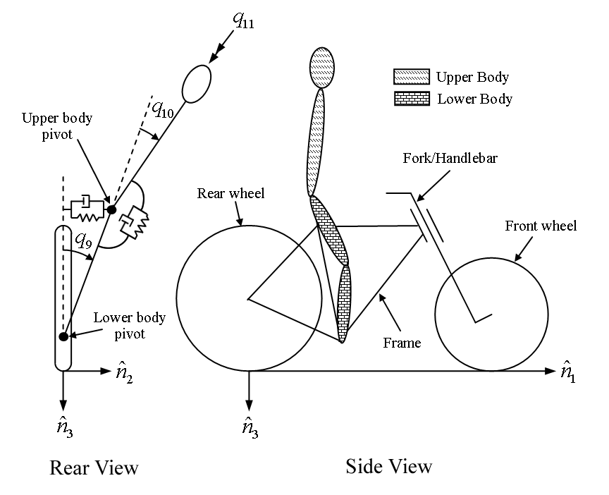
Pictorial description of (a) the additional rider degrees of freedom and (b) the six rigid bodies.
This six-rigid-body model has eleven generalized coordinates. One generalized coordinate (frame pitch) is eliminated by the holonomic configuration constraints requiring that both wheels touch the ground. This leaves ten generalized speeds, of which four are eliminated due to the nonholonomic constraints for the purely rolling wheels. The nonlinear equations of motion were linearized numerically about the nominal upright, constant velocity configuration using a central differencing method with an optimum perturbation size. The linear system is tenth order in frame roll, steer, lower body lean, upper body lean, and upper body twist.
The physical parameters are adapted from [MPRS07] with exception of the rider pivot point locations and the spring and damper constants. The pivot point locations were measured and the spring and damper constants were taken from [DLH96], which he estimated. All of the physical parameters were chosen in such a way that, if the rider degrees of freedom are locked, the model reduces to the benchmark Whipple model, similar to the later work done by [PH08b] and [SKM08].
Results and Discussion
In order to understand how the eigenvalues impact each state variable of our system, it is essential to examine the components of each eigenvector corresponding to each generalized coordinate. By detailed examination, we are able to determine how each eigenvalue contributes to each generalized coordinate, across the range of speeds examined.
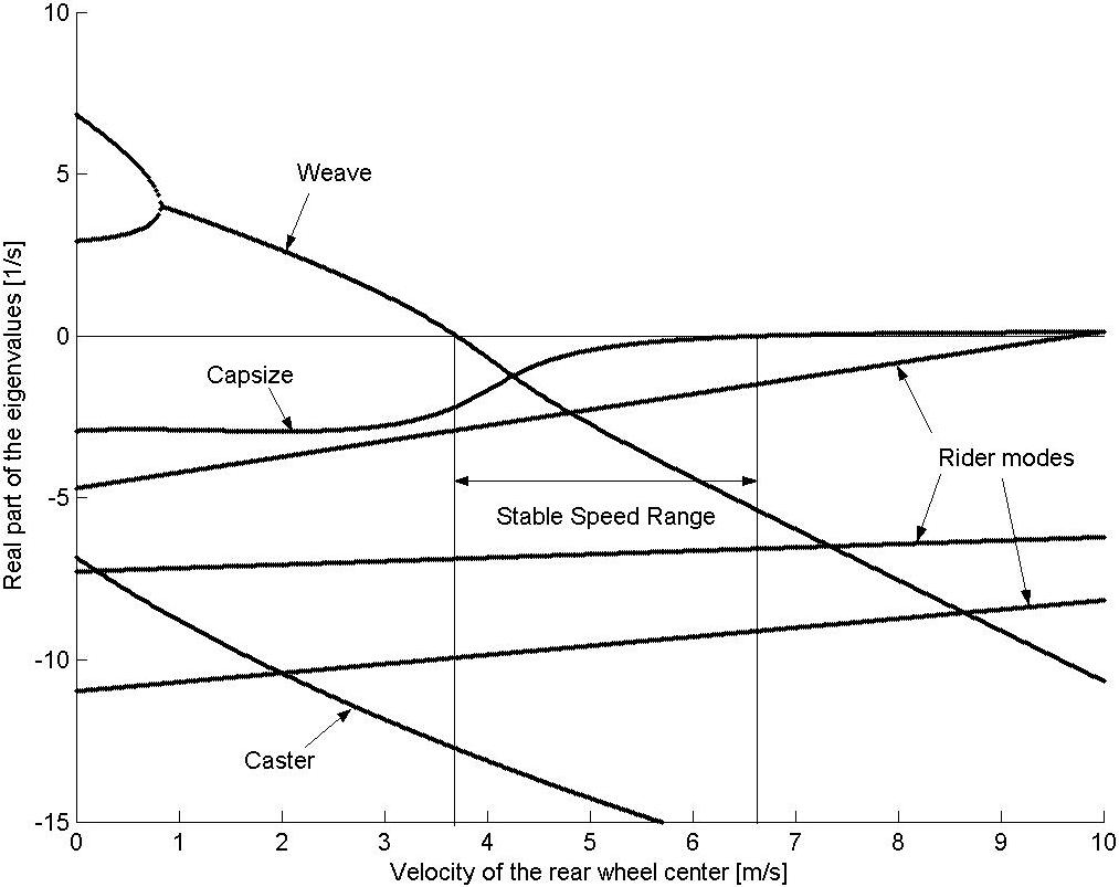
Figure 4.18 shows the real parts of the identified eigenvalues of the flexible rider model and Figure 4.19. By comparison to the Whipple model, it can be seen that the modes are greatly affected by the additional rider states. The weave mode has become unstable for all velocities and no stable speed range is present. Additionally, the rider modes are all complex at all speeds.
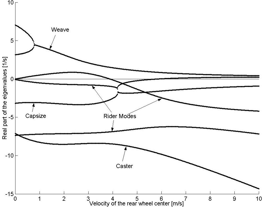
Real parts of the eigenvalues as a function of forward speed with the stiffness and damping terms set to realistic values.
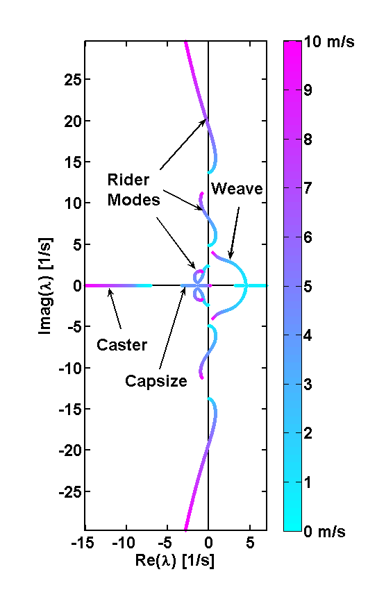
Root locus of the eigenvalues with respect to speed, a different view of Figure 4.18.
Examining the eigenvector of the weave mode at different velocities, we find that at low speeds the weave mode is dominated by frame roll and steer, while at high speeds the weave is dominated by upper body lean and twist about the body’s long axis, Figure 20. This phenomenon was also observed by Limebeer and Sharp [LS06]. Furthermore, another unstable oscillatory eigenvalue pair is present at velocities below about 4 m/s for this parameter set.
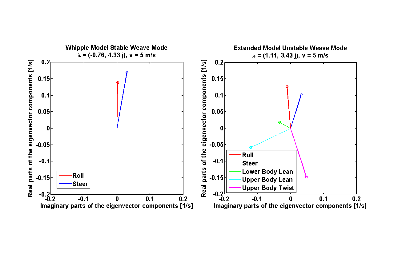
Weave mode eigenvector components for the Whipple model (left) and the de Lorenzo model (right) at 5.0 m/s.
As the stiffness and damping coefficients for the rider/frame coupling are increased (by factors of about \(10^3\) and \(30\) respectively), the eigenvalues begin to match those of the Whipple model, and a stable speed range reappears. However, the values of stiffness and damping for which a stable speed range did exist are unrealistically high Figure 21.
Real parts of the eigenvalues as a function of forward speed with the stiffness and damping terms set to unrealistically high values.
Conclusion
The notion that the bicycle-rider system can be stable during hands-free riding with no active control from the rider seems to be not necessarily true when the rider’s biomechanics are modeled more realistically. For the particular set of estimated parameters, the weave mode is unstable for the entire range of speeds investigated when realistic flexible rider dynamics are included. While the Whipple model provides many insights into the dynamics and control of the bicycle, it lacks the complexity to capture the essential dynamics that are present in open-loop hands-free riding. In particular, it is highly likely that bicycle rider must always use active control to keep the bicycle upright and self-stabilization is not guaranteed. Parameters studies that show the dependence of stability across a range of speeds for ranges of stiffness and damping at the biomechanical joints can shed more light on the system for more conclusive results.
No Hands
I’ve ended up thinking a great deal about the actual biomechanical motion one uses to balance a bicycle when riding no handed and I’ve learned much about it by talking with colleagues such as Jim Papadopoulos, Jodi Kooijman, Arend Schwab, and others. For the final studies in this dissertation I had intended to do a thorough study of the dynamics of balancing with no hands by more carefully modeling the actual biomechanics we employ during the task. Understanding hands free balancing can also shed light into how we use our body when we also have our hands on the bars, albeit with much smaller body motions because steer is almost always the optimal control input to the bicycle. Steer provides much more control authority.
It is relatively easy to learn to ride without using ones hands and many people that know how to ride a bicycle can do so. Some can even navigate roads and obstacles reasonably well. Without being able to directly affect the steering angle for control purposes, one must somehow affect the roll angle, which in turn is coupled to steering. Driving the roll angle drives the steer angle which points the bicycle in the desired direction. In the purely mechanical sense one can imagine that a rider could “lean” relative to the rear frame, thus inducing the counter reaction causing the frame to roll the opposite direction of the lean. Models are often the chosen with this theory in mind [VZ75], [PH08b], [SKM08], [Sha08], etc. They are the most intuitive and simple model but the idea of leaning may in fact be too simplistic to describe the actual biomechanical coupling a rider has with a bicycle[2].
The rider’s upper body is typically more than three times the mass of the bicycle and it takes proportionally more force to move it. The studies that will be presented in Chapters Delft Instrumented Bicycle and Motion Capture show that the rider’s upper body both moves little relative to the rear frame and leans little with with respect to inertial space[3]. In contrast the bicycle can quickly roll relative to the relatively inertially “fixed” rider. With that in mind, it is possible to imagine rolling the bicycle frame underneath the body using leg and buttock muscles. The fact that during hands-free riding one feels the seat moving back and forth under between one’s legs, gives some evidence that the coupling at the seat is important. Another interesting thing to note is that it is virtually impossible to control a bicycle without both hands and both feet placed on the grips and pedals, respectively. Removing ones feet from the pedals removes the ability to apply forces from the rider’s body to the bicycle frame, which can contribute to control of the bicycle roll angle. Secondly, it is also noteworthy that the roll angle of the bicycle can be commanded much easier when the rider is up off the seat (i.e. the rider contacts the bicycle only with hands and feet). This leads me to hypothesize that no-hand-control is dependent on the rider’s ability to roll the bicycle frame using the lower extremity muscles which are critically dependent on the leg.
If that is true, then there is may be a simple model that can capture the relative motion of the bicycle rear frame with respect to the lower extremities and pelvis. To help confirm this I examined the data from the motion capture experiments (Chapter Motion Capture) of a no-hand run with the rider pedaling. Figure 22 plots the motion of the coccyx and pelvis markers in the rear frame reference frame from the perspective of looking at the rider’s torso from the front for a single run. This plot was shows that the coccyx moves laterally with respect to bike frame, but more prevalent are the curves that the pelvis follows. This gives indication that the pelvis basically rotates about an axis just below the seat that runs longitudinally with respect to the bicycle.
The following video shows a rider balancing at 10 km/h without using his hands.
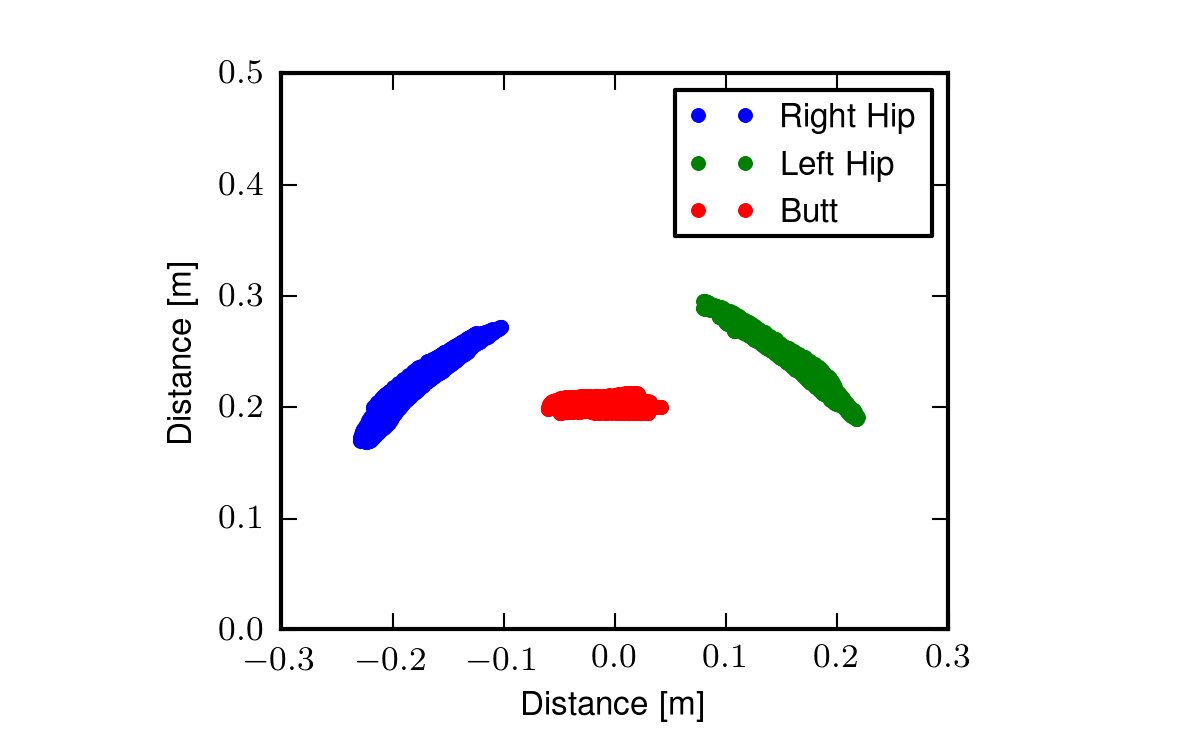
The hip trace from run # 3104. This plots the position of the two hip markers and the coccyx marker relative to the bicycle’s rear frame in space over time. View the video.
Gilbert Gede and I began devising a harness that would both constrain the rider’s motion to the motion observed in Figure 22 and allows us to measure the forces and the kinematics involved. We created a video shot from behind and shows me balancing no-handed on a treadmill. We taped three sticks to my back: one across the shoulders, the second to the upper portion of my spine, and the third to the lower portion of my spine to visualize the dominant motion of the rider with respect to the bicycle frame and how the spine moved. I chose the stick locations based on the motion capture studies we did. This video confirmed that the spine bend could probably be described by a single joint in the middle of the spine and that the pelvis rolls about the seat (i.e. a longitudinal axis just below the seat).
The following video demonstrates that the bicycle frame does roll relative to the somewhat inertially fixed rider, that the hips rotate about the seat and also that the spine may only need one laterally rotational degree of freedom to capture the dominate spine motions.
At this point, we constructed a mock-up of a harness that would both measure these motions and limit the rider to the observed motions.
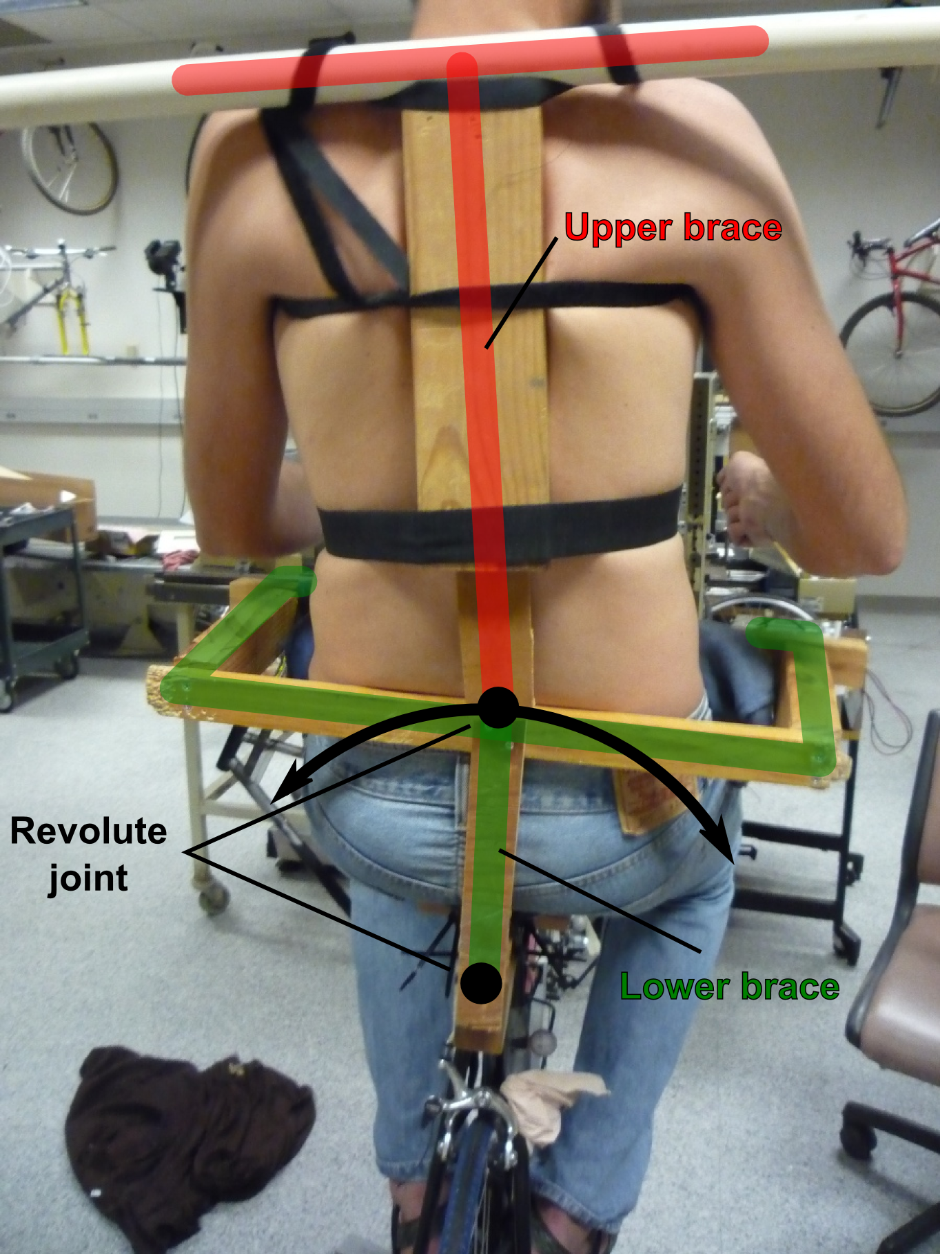
A mock-up of a harness to measure the dominant motions of the rider’s pelvis roll angle relative to the bicycle rear frame and the lean angle relative to the pelvis. The lower brace (green) is affixed the rider’s pelvis and rotates relative to the bicycle frame. The second joint allows the rider’s torso to lean relative to the pelvis.
The model to describe this motion would have a revolute joint just below the seat such that the riders pelvis can roll about a longitudinal revolute joint just below the seat. The legs would be constrained such that the feet locked into the foot pegs and the knee angles would be dependent on the pelvis roll angle. Finally, the spine would be stiffened with a back brace and a single revolute joint for back lean relative to the pelvis would be measured.
We intended to develop a harness and pair it with a force measuring seat post and foot pegs which measure the downward force applied by the feet to the bicycle. The goal would have been to characterize the both the kinematic and kinetic coupling between the rider and the bicycle which causes the bicycle to roll. I included this section to simply document the thoughts and effort, but none of this was ever executed in a proper experiment.
Conclusions
Several extensions to the Whipple model have been presented. The details are not exhaustive but provide some useful conclusions for the coming chapters. I showed that the lateral force input we used in the control experiments must be properly accounted for and not simply assumed to be characterized by a pure roll torque. This force contributes to both the roll and steer degrees of freedom which is a function of the location of the force application. Secondly, the addition of the inertial affects of the arms change the bicycle system dynamics significantly. In this particular case, it eliminates any possibility for stability and the capsize mode becomes very unstable. This model will play a role in the data analysis presented in Chapter System Identification because it more realistically models our test subjects’ motion. In the third section, I show how adding a flywheel to the front wheel of a bicycle can radically change it’s stable speed regime and can make the model stable at very low speeds, even slower than average walking. But if the inertial effects of the rider are taken into account, the flywheel may have to spin at very high speeds for any significant change in dynamics. Next, I show that adding various rider degrees of freedom generally creates an unstable system, but passive forces acting on the new joints can potentially stabilize the new modes. It is likely that the rider must make use of a combination of both passive and active control to keep the bicycle/rider system stable. Finally, I’ve presented some ideas and thoughts on developing a slightly different biomechanical model of the rider that may be a more realistic way of characterizing the motion used for hands-free control of the bicycle.
Footnotes
| [1] | We got a kick out of “crotch stiffness” i.e. the stiffness of the crotch spring, and tried to encourage Mont to use the terminology when he presented this for us in Taiwan. |
| [2] | A model for leaning on a motorcycle makes more sense as the mass of the motorcycle is comparable to or more than the mass of the riders upper body. |
| [3] | [WZT79] points out this with respect to motorcycles, in that the rider’s upper body mostly stays still and rider’s lean angle is nearly equal and opposite to the motorcycle. |
