Lab Report Guidelines
Lab reports prepared for EME 171 should meet the following guidelines:
- One lab report per group.
- Lab reports must be submitted online on Canvas. You may scan or take pictures of hand-calculations or hand-drawn figures (such as bond graphs) to include them in the report.
- Start each report with a title page containing the following information:
- Lab assignment name & number
- Course
- Quarter
- Year
- Date
- Your names
- Student IDs
- Include a brief introduction explaining the system, simulation, and learning objectives.
- Reports must include the bond graph, the equations of motion, and the parameters used.
- Reports must include a list of the system's states and parameters, and must clearly explain any computed values such as time parameters, initial conditions, and derived parameters.
- Use both text and plots to explain your work and findings and to answer the questions presented in the lab. Write the report such that a reader can understand the topic given only your document. All results should be explained with text (complete sentences and paragraphs) interwoven among the figures that you present.
- Be sure to use clear, concise language. Omit needless words. Grammar, spelling, conciseness, structure, organization, and formatting will be assessed.
- All plots should have:
- Axes labeled with units
- Axes limits set to show the important aspects of the graph
- Fonts large enough to read (>= 8pt)
- A figure number, short title, and caption explaining what the figure is
- Legends to describe multiple lines on a single plot
- Include your code in the report in an appendix.
- Show each function and the main script. These should be monospaced font formatting and ideally syntax highlighted. You can use the publish function in Octave and Matlab to export code files to nice formats. See https://www.mathworks.com/help/matlab/matlab_prog/publishing-matlab-code.html (Links to an external site.) for more information.
- Your code should be readable by someone else. Include comments, useful variable names, and follow good style recommendations, for example see this guide. Imagine that you will come back to this in 10 years and you want to be able to understand it quickly.
- All functions should have a "help" description written in the standard style describing the inputs and outputs of the function which is customized for your particular function design. This template is useful (click the function tab).
Example Lab Report
Cover Page
| Lab 1: Introduction to Simulation |
| EME171 - Analysis, Simulation and Design of Mechatronic Systems |
| Fall 2019 |
| October 18, 2019 |
| Student A -- 123456789 |
| Student B -- 987654321 |
Introduction
Introduce the lab material. This includes describing the system you are simulating, providing the system diagram, bond graph, state and output equations, and parameters, discussing the learning objectives, and so on. In this example, the lab concerns the simulation of a nonlinear mass/spring/damper system subjected to a force input, where the nonlinear spring has a constitutive law
The goal of this lab is to linearize the spring and to demonstrate the effects of linearization on simulation accuracy. The system and bond graph are shown in Figure 1.
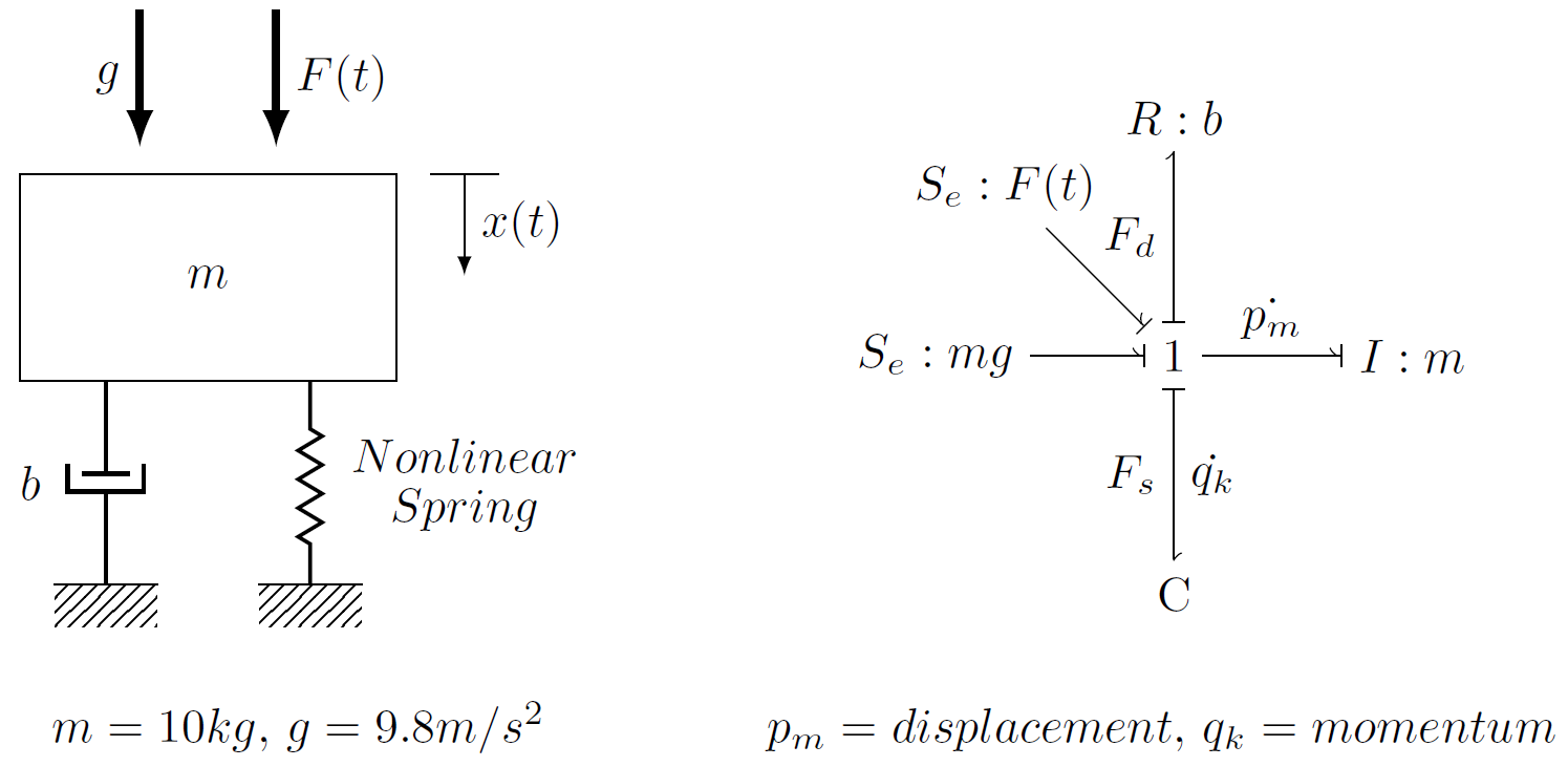
Figure 1: Mechanical Schematic of Nonlinear System (left) and equivalent bond graph (right).
The state equations for the nonlinear system are:
The state equations for the linearized system are:
where \(p_{m}\) is the momentum of the mass, \(q_{k}\) is the spring displacement, \(G\) is the nonlinear spring coefficient, \(k\) is the linearized spring coefficient, \(b\) is the damping coefficient, \(m\) is the mass, and \(F(t)\) is the input force.
Additionally, the output of this simulation is the deflection from equilibrium \(\delta\), where
Calculations
In this section, show your work for any computed variables like initial conditions, equilibrium points, or computed parameters. Make sure to include these here even if the calculations are present in your code. You may include scanned images of hand computations if need be. In this example, we have a section for computing system parameters and time parameters, but these will of course vary with each lab.
System Parameters
A mass \(m=10\) kg is lowered onto a nonlinear spring and damper and reaches its equilibrium position at \(q_{k,eq}=0.25\) m. Knowing this, the nonlinear spring constant \(G\) can be found:
The linearized spring stiffness can be found by taking the derivative of the spring force equation at the equilibrium point.
We can approximate the natural frequency from the linearized spring constant and the mass as
From a given damping ratio of \(\zeta=0.3\) we can find the damping coefficient
Time Parameters
Be sure to include a section for your calculations for the time parameters; that is, how you computed the final time and the number of time steps. Even if this work is present in your code, be sure to show it here as well.
Simulation
In this section, discuss what you simulated and the ensuing results. Use both text and plots to explain your work and findings and to answer the questions presented in the lab. Write the report such that a reader can understand the topic given only your document. All results should be explained with text (complete sentences and paragraphs) interwoven among the figures that you present. Remember to clearly label the elements of plot, including axes, axes labels, titles, and captions. Also, if you have multiple plots on the same graph, make sure they are visually distinct.
The linear and nonlinear equations of motion were simulated for \(F/mg =\) 0.1, 0.2, 2.0, and 5.0. The results of these simulations are shown below. In all cases, the linearized model overestimated the system's displacement. This is because the actual spring force increased much more rapidly than the spring force of the linearized model (specifically, cubic growth vs. linear growth). Additionally, the linearized model kept a constant natural frequency, while the response frequency of the nonlinear system increased with displacement. Again, this discrepancy is due to the linearized model not accounting for the actual system's increasing stiffness.
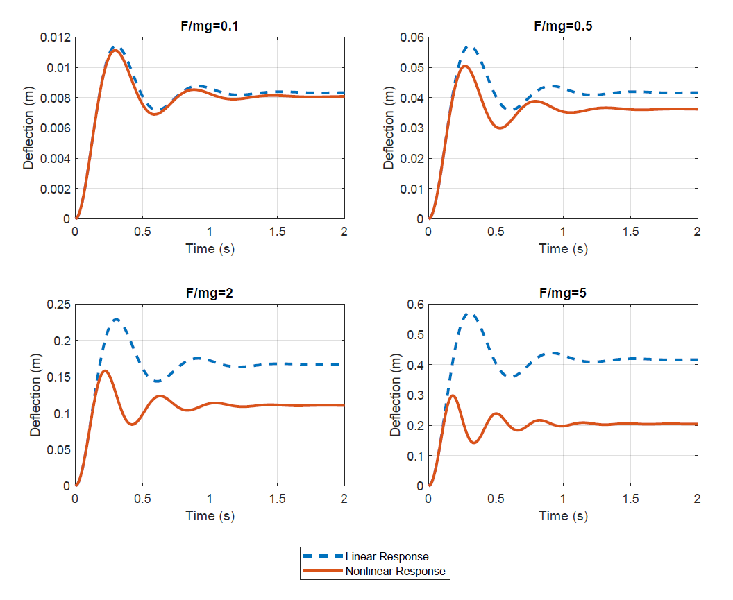
Figure 2: Comparison of results for the nonlinear and linearized deflections.
Contributions
It is expected that each student contributes equitably in all aspects of the solutions to the lab and project assignments. We expect to see that each student did model development, coding, writing, interpretation, etc. In this section, describe in several sentences what the contributions of each lab partner was for the assignment. Here is an example:
Laurel set up the first model for this report. Feng created the input and forcing functions for the model. Following the first analysis, both team members attempted to solve the free body diagrams and create equations of motion to confirm the correct model. Both members coded their own individual versions to compare elements that did and did not work. Each member troubleshooted code for the other when they became stuck. Laurel wrote the introduction and Feng wrote the conclusion. Laurel wrote the model description and Feng drew the diagrams in that section. Both wrote the results section.
Code
Include all code at the end of your report. Your code should be well-commented, and any function files you write should include a standard "help" description written in the standard style describing the inputs and outputs of the function.
The example code shown below does not correspond to the system above, provides an example of what yours submitted code should look like. Make sure it is in a fixed-width font and (ideally) has syntax highlighting.
Simulation Script
% integrate the ODEs as defined above
x0 = [5*pi/180; 0];
ts = linspace(0, 10, 500);
p.m = 1;
p.l = 1;
p.g = 9.81;
f_anon = @(t, x) eval_rhs_with_input(t, x, @eval_input, p);
[ts, xs] = ode45(f_anon, ts, x0);

% to compute the outputs at each time, loop through time evaluating f(t, x,
% r, p) and then h(t, x', x, r, p)
zs = zeros(length(ts), 2);  % place to store outputs
for i=1:length(ts)
    % calculate x' at the given time
    xdot = eval_rhs_with_input(ts(i), xs(i, :), @eval_input, p);
    % calculate the outputs that depend on x' and store them
    zs(i, :) = eval_output_with_state_derivatives(ts(i), xdot, xs(i, :), @eval_input, p);
end
Input Function
function r = eval_step_input(t, x, p)
% EVAL_STEP_INPUT - Returns the input vector at any given time.
%
% Syntax: r = eval_step_input(t, x, p)
%
% Inputs:
%   t - Scalar value of time, size 1x1.
%   x - State vector at time t, size mx1 where m is the number of states.
%   p - Constant parameter structure with p items where p is the number of
%       parameters.
% Outputs:
%   r - Input vector at time t, size ox1 where o is the number of inputs.

% NOTE : x and p are not used in this case

% calculate the step input
if t > 1.0
    tau = 0.5;  % [N]
else
    tau = 0.0; % [N]
end

% pack the input values into a ox1 vector
r = [tau];

end
State Equations Function
function xdot = eval_rhs_with_input(t, x, w, p)
% EVAL_RHS_WITH_INPUT - Returns the time derivative of the states, i.e.
% evaluates the right hand side of the explicit ordinary differential
% equations.
%
% Syntax: xdot = eval_rhs_with_input(t, x, w, p)
%
% Inputs:
%   t - Scalar value of time, size 1x1.
%   x - State vector at time t, size mx1 where m is the number of states.
%   w - Anonymous function, w(t, x, p), that returns the input vector at
%       time t, size ox1 were o is the number of inputs.
%   p - Constant parameter structure with p items where p is the number of
%       parameters.
% Outputs:
%   xdot - Time derivative of the states at time t, size mx1.

% unpack the states into useful variable names
theta = x(1);
omega = x(2);

% evaluate the input function
r = w(t, x, p);

% unpack the inputs into useful variable names
tau = r(1);

% unpack the parameters into useful variable names
m = p.m;
l = p.l;
g = p.g;

% calculate the state derivatives
thetadot = omega;
omegadot = (-m*g*l*sin(theta) + tau)/(m*l^2);

% pack the state derivatives into an mx1 vector
xdot = [thetadot; omegadot];

end
Output Function
function y = eval_output(t, x, r, p)
% EVAL_OUTPUT - Returns the output vector at the specified time.
%
% Syntax: y = eval_output(t, x, r, p)
%
% Inputs:
%   t - Scalar value of time, size 1x1.
%   x - State vector at time t, size mx1 where m is the number of states.
%   r - Input vector at time t, size ox1 where o is the number of
%       inputs.
%   p - Constant parameter structure with p items where p is the number of
%       parameters.
% Outputs:
%   y - Output vector at time t, size qx1 where q is the number of outputs.

% unpacke the states
theta = x(1);
omega = x(2);

% unpack the parameters
m = p.m;
l = p.l;
g = p.g;

% calculate the Cartesian position of the pendulum bob
x_pos = l*sin(theta);
y_pos = l - l*cos(theta);  % position relative to stable equilibrium

% calculate the kinetic and potential energies
kinetic_energy = m*l^2*omega^2/2;
potential_energy = m*g*y_pos;

% pack the outputs into a qx1 vector
y = [x_pos; y_pos; kinetic_energy; potential_energy];

end
Output Function with State Derivatives
function z = eval_output_with_state_derivatives(t, xdot, x, r, p)
% EVAL_OUTPUT_WITH_STATE_DERIVATIVES - Returns the output vector at the
% specified time.
%
% Syntax: z = eval_output_with_state_derivatives(t, xdot, x, r, p)
%
% Inputs:
%   t - Scalar value of time, size 1x1.
%   xdot - State derivative vector as time t, size mx1 where m is the number
%          of states.
%   x - State vector at time t, size mx1 where m is the number of states.
%   r - Input vector at time t, size ox1 were o is the number of inputs.
%   p - Constant parameter structure with p items where p is the number of
%       parameters.
% Outputs:
%   z - Output vector at time t, size qx1.

% unpack all of the vectors
thetadot = xdot(1);
omegadot = xdot(2);

theta = x(1);
omega = x(2);

m = p.m;
l = p.l;
g = p.g;

% calculate the radial and tangential accelerations
radial_acc = omega^2 * l;
tangential_acc = omegadot * l;

% pack the result into a qx1 vector
z = [radial_acc; tangential_acc];

end