
- Fri 01 November 2013
- misc
- Jason K. Moore
- #pydy, #python, #code generation, #multibody dynamics, #ordinary differential equations
I've been working on implementing a walking simulation model that is based on and compatible with a model developed by my PI, Ton van den Bogert, in http://dx.doi.org/10.1016/j.jbiomech.2009.12.012. Ton provided me with source code that that derives the equations of motion for the 2D walker, which I will be making publicly available soon. His tool chain is primarily based on closed proprietary software, i.e. Autolev and Matlab. I didn't have it in me to use those tools since we've spent so much time and effort developing a workflow for these kinds of problems with PyDy, so I did what any idealistic young scientist would do and rewrote Ton's model with an open source tool chain. In the process, I needed to improve the code generation capabilities we were relying on for the PyDy workflow and have a small step in improvements on that front.
We are primarily interested in generating numerical code from SymPy's symbolic expressions which are stored in two matrices that generalize a set of first order coupled differential equations. The LagrangesMethod and KanesMethod classes in the mechanics package generate symbolic ordinary differential equations for multibody systems in this form:
where \(x\) is a vector of the system states, \(M\) is the mass matrix, which may or may not be identity, and \(F\) is a forcing vector. The mathematical expressions in \(M\) and \(F\) are non-linear functions which generally consist of common operations: addition, multiplication, trigonometric functions, absolute values, exponentiation, piecewise functions, etc. For complex systems, the expressions that make up the entries of \(M\) and \(F\) can be thousands of operations long.
Most numerical ODE integration routines require that the ODE's are in first order form and are explicit in \(\dot{x}\). There are generally two major computational steps in the integration process for our systems:
- Evaluation of the expressions contained in \(M\) and \(F\).
- Solving for \(\dot{x}\).
For systems without velocity constraints, \(M\) is \(2n\times2n\) matrix where \(n\) is the number of degrees of freedom of the system. The complexity of the entries of \(M\) and \(F\) are a function of the system complexity: number of bodies/particles, number and types of forces, number of physical parameters, etc. Whether or not step 1 or 2 is more computationally intensive depends on the problem, so in general we need to make both as fast as possible to achieve at least real time simulation speeds.
For step 2, we rely on canned numerical linear system solvers. In general LU decomposition, i.e Gaussian elimination, is used but Cholesky Decomposition can be used for certain classes of systems. Gaussian elimination has a computational complexity of \(O((2n)^3)\) for our systems without velocity constraints where there are \(n\) dynamical differential equations and \(n\) kinematical differential equations. In many cases, \(M\) is symmetric positive definite and can be solved with Cholesky decomposition for half the computational cost of Gaussian elimination.
In general, we rely on software such as LAPACK for these routines which offer good computational speed. But the evaluation of the symbolic expressions is a different story. The three things we are most concerned with respect to the long expression evaluation are:
- Simplification
- Common sub expressions
- Speed evaluation of long expressions
Simplification
Simplification, in particular trigonometric simplification, can reduce the resulting expressions significantly. We'd love to use simplification routines extensively but the issue with this is that symbolic simplification is a difficult problem for large expressions. The algorithms don't offer computational speed that allows a for real time workflow. SymPy recently implement Fu's trigonometric simplification method, but it still hangs, in terms of speed, on many of our large expressions.
Common sub expressions
We've typically concerned ourselves with finding common sub expressions in our large expressions. For example, if we compute \(cos(q(t))\) 1000 times, then we should compute it once and store the result in a variable:
z_0 = cos(q)
expression = z_0 * z_0 + z_0 + z_0 ** 2
This generally seems like a good idea, but it may be fruitless for compiled languages because compilers are optimized to do this sort of thing anyways. But it may be useful for high level code generation. SymPy s cse() function recently got a speed boost, but there is still work to be done on creating sub expressions of combinations of sub expressions that could reduce the computational time.
Speed
Fast evaluation of long expressions generally requires getting closer metal. C and Fortran are likely the best options for speedy numerical evaluation of these expressions. The best solution will likely rely on low level code and compilation.
The package
The package I'm tinkering with explores some options for these methods. Currently, it generates code to evaluate \(M\) and :math`F` with three methods: sympy.utilities.lambdify.lambdify, sympy.printing.theancode.theano_function, and sympy.printing.ccode + Cython.
lambdify
SymPy's lambdify prints the expression tree to a python lambda function. This has very fast code generation times, but numerical evaluation is extremely slow for long expressions.
Theano
Theano is a python symbolic to numerical code generator. Theano can output code to run on the CPU or GPU and can generate code that includes numerical operations such as solving linear systems. Matthew Rocklin created a bridge from SymPy expression trees to Theano expression trees to allow easy code gen with Theano from SymPy, 1.
C
Finally, SymPy offers expression to C code printing, sympy.printing.ccode, that is useful to writing custom code generators in C. Their codegen module makes use of the printer to make compilable functions and the autowrap module allows easy wrapping for use in Python, but these do not support Matrix evaluations, yet. So I wrote a custom C code generator and auto generated Cython wrapper for the matrix/vector evaluations we need. It works like this:
- Generate a custom C function which computes the mass matrix and forcing vector
- Wrap it with Cython using NumPy types.
- Compile the code.
- Evaluate the \(M\) and \(F\) functions numerically.
- Solve for \(\dot{x}\) using numpy.linalg.solve.
These are the resources I used to learn about Cython and NumPy use:
- Nice example on Stack Overflow: http://stackoverflow.com/questions/3046305/simple-wrapping-of-c-code-with-cython
- Cython docs: http://docs.cython.org/src/tutorial/numpy.html and http://docs.cython.org/src/userguide/numpy_tutorial.html
- The SciPy lecture notes on interfacing with C: http://scipy-lectures.github.io/advanced/interfacing_with_c/interfacing_with_c.html
- Travis Oliphant's blog post comparing Cython, Weave, and NumPy: http://technicaldiscovery.blogspot.com/2011/06/speeding-up-python-numpy-cython-and.html
Cython Code
Here is the example C code and the Cython wrapping for a simple 1 DoF mass, spring, damper system under the influence of gravity and an external force. First the C code, mass_forcing_c.c (make sure to name this different than you desired Cython module name or it will be overwritten), and the header file, mass_forcing_c.h:
#include <math.h>
#include "mass_forcing_c.h"

void mass_forcing(double constants[4], // constants = [m, k, c, g]
                  double coordinates[1], // generalized_coordinates = [x]
                  double speeds[1], // generalized_speeds = [v]
                  double specified[1], // external = [F]
                  double mass_matrix[4], // computed
                  double forcing_vector[2]) // computed
{
    // common subexpressions
    double z_0 = speeds[0];

    // mass matrix
    mass_matrix[0] = 1;
    mass_matrix[1] = 0;
    mass_matrix[2] = 0;
    mass_matrix[3] = constants[0];

    // forcing vector
    forcing_vector[0] = z_0;
    forcing_vector[1] = -constants[2]*z_0 + constants[3]*constants[0] - constants[1]*coordinates[0] + specified[0];
}
void mass_forcing(double constants[4], // constants = [m, k, c, g]
                  double coordinates[1], // generalized_coordinates = [x]
                  double speeds[1], // generalized_speeds = [v]
                  double specified[1], // external = [F]
                  double mass_matrix[4], // computed
                  double forcing_vector[2]); // computed
I simply stored \(M\) as a flat array. It may be better to stored it as a 2D array so that I don't need a reshape() call in the Cython wrapper. I also store all of the inputs as arrays. It could make sense to stored the some or all of them in structs so that we could access them be name instead of indice.
The mass_forcing.pyx file declares the contents of the header file and defines a function for easy use in Python. The types are pinned to the NumPy C API definitions for 1D continous arrays. I could potentially avoid defining arrays of zeros for initialization by passing in empty or zero arrays and the reshaping step on the output. Both of those could potentially speed things up.
import numpy as np
cimport numpy as np

cdef extern from "mass_forcing.h":
    void mass_forcing(double constants[4],
                      double coordinates[1],
                      double speeds[1],
                      double specified[1],
                      double mass_matrix[4],
                      double forcing_vector[2])


def mass_forcing_matrices(np.ndarray[np.double_t, ndim=1] constants,
                          np.ndarray[np.double_t, ndim=1] coordinates,
                          np.ndarray[np.double_t, ndim=1] speeds,
                          np.ndarray[np.double_t, ndim=1] specified):

    assert len(constants) == 4
    assert len(coordinates) == 1
    assert len(speeds) == 1

    cdef np.ndarray[np.double_t, ndim=1] mass_matrix = np.zeros(4)
    cdef np.ndarray[np.double_t, ndim=1] forcing_vector = np.zeros(2)

    mass_forcing(<double*> constants.data,
                 <double*> coordinates.data,
                 <double*> speeds.data,
                 <double*> specified.data,
                 <double*> mass_matrix.data,
                 <double*> forcing_vector.data)

    return mass_matrix.reshape(4, 1), forcing_vector.reshape(2, 1)
Finally, I use the disutils method of building the shared object file which can be imported into Python. Here is the mass_forcing_setup.py file:
import numpy
from distutils.core import setup
from distutils.extension import Extension
from Cython.Distutils import build_ext

ext_modules = [Extension(
                name="mass_forcing",
                sources=["mass_forcing.pyx", "mass_forcing.c"],
                include_dirs=[numpy.get_include()],
                )]

setup(
    name="mass_forcing",
    cmdclass = {'build_ext': build_ext},
    ext_modules = ext_modules,
)
To buid the extension simple type:
$ python mass_forcing_setup.py build_ext --inplace
And you can import and use the function:
>>> import mass_forcing
>>> from numpy.random import random as r
>>> mass_matrix, forcing_vector = mass_forcing.mass_forcing_matrices(r(4), r(1), r(1), r(1))
Benchmark Problem
Once I got this all working, I used the 2D n-link pendulum as a benchmark problem to test the three methods. Each link adds a degree of freedom to the system and it doesn't take long for the equations to get real hairy. The benchmark times the derivation of the symbolic equations of motion and for each of the backends it times both the code generation and the integration steps. The results from my computer for 1 to 20 links in the pendulum are shown in this plot:
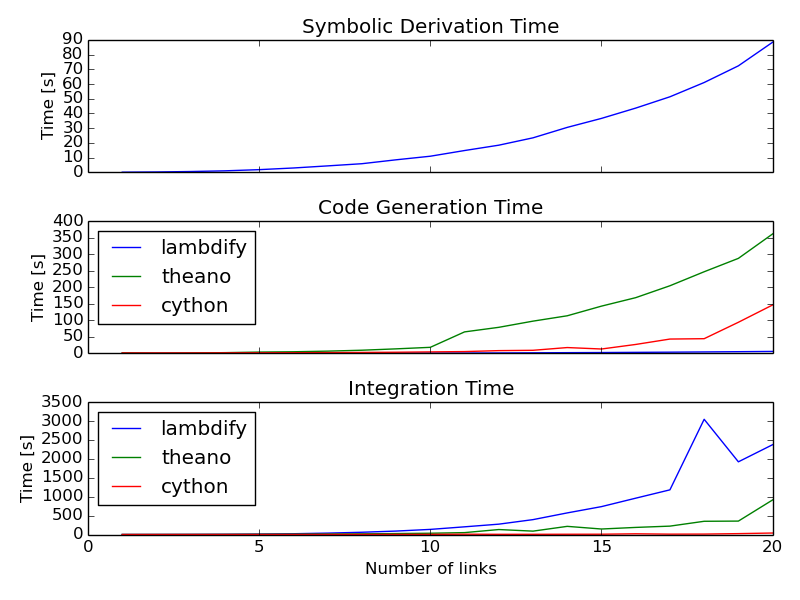
The print out shows the exact time values. For 1000 time steps of integration over 10 seconds of real time (100 hz) for the 20 link problem, the Cython method wins out at 39 seconds. Theano took 914 seconds (23x slower) and lambdify took 2374 seconds (60x slower). Cython was able to integrate the equations of motion for up to 17 links at real time speeds (9.5 seconds) for 100hz throughput. The timing was dependent on my system processes, so there are some blips. It'd be nice to get an average of this computation. You can run the benchmark yourself here:
https://github.com/PythonDynamics/pydy-code-gen/blob/master/misc/benchmark.py
These are some general observations:
- Lambdify generates the code very fast.
- Theano takes more time to generate code than lambdify, but is significantly faster at evaluation in the integration step.
- The Cython wrapped C code evaluates extremely faster than both methods and doesn't take to long to generate the code.
- The derivations are pretty fast, with the 20 link pendulum taking 88 seconds. I'm looking forward to trying out Ondřej's csympy implementation for this, which could get derivations down to second speeds.
The package and benchmark code are hosted here:
Conclusion
There is a great deal of improvement needed for this package, but I think it demonstrates a proof of concept that we can generate fast code that can still be used at the high level. We'd ideally like the derivation + simulation time to take no more than 20 seconds for relatively complex problems to expect this to be used for any kind of backend to a GUI based model builder. That may be too much to expect though, as purely numerical \(O(n)\) methods for multibody dynamics are still superior for this.