Delft Instrumented Bicycle
Preface
I had contacted the authors of [MPRS07] in the early winter of 2006 to try to get some tips on where to go with my master’s thesis, which I wanted to do on the handling qualities of bicycles. I had previously come across Arend, Jaap, and Jim’s conference paper [SMP04] on their benchmark Whipple model and used it to help me build and validate my first model earlier that year. Andy, Jim, and Arend all replied, Jim at great length as usual, and the seeds were sown for some future collaboration. Jim began flooding my inbox with years of thoughts on the handling of bicycles and it turned out that Arend had just applied for a big grant to fund two PhD students for bicycle handling research that was uncannily similar to what I was dreaming up myself. I hadn’t decided to do my PhD at UC Davis quite yet and Arend’s potential PhD slot was enticing (Jodi was slated for one). But I ended up finishing my masters the following spring and signing on for the PhD at Davis. That summer I started thinking about applying for a Fulbright grant to study somewhere. I contacted Arend again to see if he was interested in having me and he was excited. I told him I was going to do it and then put it off. A week shy of the deadline, I told Arend I didn’t have time to do it. He encouraged me to apply anyway and I agreed to push through. I spent the next week putting together the proposal full time and after several drafts I sent it off. I didn’t think about it much after that, but luck was on my side and I received the acceptance letter from the Fulbright commission the following spring. I was headed to the Netherlands for my first time living abroad. In the meantime Arend found a way to fund a PhD for Jodi so there was going to be some momentum and a teammate when I arrived.
When I arrived in Delft at the end of August in 2008 Jodi was working on several projects: a bicycle handling qualities review paper [KS11], the two mass skate bicycle [KMP+11], and an instrumented bicycle. I helped to some degree with all the projects, but primarily with setting up the instrumented bicycle and planning a set of experiments. This chapter details the work we did with the first instrumented bicycle. I’ve taken the text directly from our conference paper [KSM09] and gone through it with some updates, clarifications, and additions. Jodi and Arend were the primary writers of the paper. My contributions were more of the experimental design, performing the experiments, analyzing the data, discussing results and working on a visualization graphical interface that we never really used due to the inability to synchronize the video data we took with the sensor data.
Abstract
The purpose of this study is to identify human control actions in normal bicycling. The task under study is the stabilization of the mostly unstable lateral motion of the bicycle-rider system. We studied this by visual observation of the rider and measuring the vehicle motions. The observations show that very little upper-body lean occurs in normal riding and that stabilization is done primarily maintained by steering control actions. However, at very low forward speed a second control action was observed: knee movement. Moreover, the frequency of the control actions are all dominated by the pedaling frequency, while the amplitude of the steering motion increases rapidly with decreasing forward speed.
Introduction
Riding a bicycle is an acquired skill. At very low speeds the bicycle is very unstable and requires great attention by the rider. However, at moderate speed the bicycle is easy to stabilize, often with little conscious thought by the rider. These observations are corroborated by a stability analysis on a simple dynamical model of an uncontrolled bicycle [MPRS07] and some experiments [KSM08] and [KS09]. Although there is little established knowledge on how a person stabilizes a bicycle, two basic features are known: some uncontrolled riderless bicycles can balance themselves given some initial speed, and one can balance a forward moving bicycle by turning the front wheel in the direction of the undesired lean. But we all know that a rider on a bicycle not only moves the handlebars but also may make use of their upper body and other extremities. These rider body motions are even more profound when riding a motorcycle in extreme maneuvers [CL02].
The purpose of this study is to identify the major human control actions in normal bicycling focusing on the stabilization task.[1] We use the term “normal” to describe casual bicycling that requires minimal conscious control. The identification is done by visual observation of the rider and measurement of the motions of the instrumented bicycle, see Figure 7.1. In order to observe the human control actions a number of experiments were carried out. First, a typical town ride was performed to investigate what sort of actions take place during casual riding through an urban environment. After this, experiments were carried out in more controlled environment, a large treadmill (3 × 5 m), at various speeds. The same bicycle was used during all the experiments. The bicycle was ridden by two averagely skilled riders. Three riding cases were considered: normal bicycling, bicycle without pedaling (towing), and normal bicycling with lateral perturbations. These experiments were carried out to identify the upper body motions and the effect of the pedaling motion on the control. The rider was told to simply stabilize the bicycle and to generally ride in the longitudinal direction of the treadmill; no tracking task was set. Recorded data included the rigid body motions of the bicycle rear frame and the front assembly. The rider motion relative to the rear frame was recorded via video.
Instrumented Bicycle
A standard Dutch bicycle, 2008 Batavus Browser, was chosen for the experiments and is shown in Figure 7.1. This is a bicycle of conventional design, fitted with a 3-speed SRAM rear hub and coaster brakes. Some of the peripheral components were removed in order to be able to install measurement equipment and sensors (see Table 7.1). The bicycle was equipped with a 1/3” CCD color bullet-camera with 2.9mm (wide angle) lens. The camera was located at the front and directed towards the rider and rotated 90 degrees clockwise to get portrait aspect ratio. The video signal was recorded, via the AV-in port, on DV tape of a Sony Handycam located on the rear rack of the bicycle. The bullet camera was placed horizontally, approximately 65 cm in front of the handlebars and 1.2 m above the ground and held in place by a carbon-fiber boom connected to the down-tube of the rear frame, see Figure 7.1. This allowed us to view the rider’s motion with respect to the bicycle frame.

The instrumented bicycle with camera boom and video camera lens (1). On the rear rack the measurement computer (2), video camcorder (3) and battery packs (4) are positioned. Measured signals are the steer angle and steer-rate (5), rear frame lean- and yaw-rate (6) and forward speed (7).
| Measurement | Sensor Type | Manufacturer | Type | Specification |
|---|---|---|---|---|
| Yaw, roll, steer rates | MEMS Angular Rate | Silicon Sensing | CRS03 | Full range output \(\pm\) 100 deg/s |
| Steer angle | Potentiometer | Sakae | FPC40A | 1 turn, conductive plastic, Servo mount |
| Forward speed | DC-motor | Maxon | 2326-940-12-216-200 | Graphite brush motor with a 5cm diameter disk on the shaft |
| Cadence | Reed relay and magnet | Kitchen magnet |
We used a National Instruments CompactRIO (type CRIO-9014) computer for data collection. The CompactRIO was installed on the rear rack of the bicycle. It was fitted with a 32-channel, 16 bit analogue input module and a 4-channel, 16 bit analogue output module as well as a CRIO WLAN-MH1000 wireless modem by S.E.A. Datentechnik GmbH for a wireless connection with a “ground station” router, to which a laptop was connected. The measurement system is able to run autonomously once a measurement sequence is initiated. The CompactRIO was powered by a 11.1V, 1500 mAh Lithium Polymer battery which was also placed on the bicycle’s rear rack.
The recorded signals were the body fixed roll, yaw, and steer rates, the steer angle, the rear wheel speed, and the pedaling cadence frequency. The angular rates were measured using 3 Silicon Sensing CRS03, single axis angular rate sensors with a rate range of ± 100 deg/s. The steer angle was measured using a potentiometer placed on the rear frame against the front of the head tube and connected via a belt and pulley pair. The angular rate sensors and the angular potentiometer were powered by a 4.8V, 2100 mAh Nickel Cadmium battery. The forward speed was measured by measuring the output voltage of a Maxon motor that was driven by the rear wheel. The cadence frequency was measured by a reed relay placed on the rear frame, and a magnet placed on the left crank-arm.
Town Ride Experiment
Our first basic experiment was a short, 15 minute ride around town. This experiment took place under normal riding conditions (dry weather, day-light, etc.), on roads familiar to the rider. The course covered included a round-a-bout, dedicated cycling paths, speed-bumps, pavement, normal tarmac roads, tight bends in a residential area and the rider had to stop at a number of traffic lights. There were no special precautions taken and the experiment was carried out amongst other traffic. From the recorded video and sensor data two main observations were made:
- The video data showed that there was very little upper body lean relative to the rear frame during the entire ride. The small relative upper body lean that was noted appeared to simply be a result of pedaling. Only in the last few seconds prior to a sharp corner was an upper body lean angle observed, indicating that the lean was carried out because of a sudden heading change.
- The recorded data, part of which is shown in Figure 7.2, clearly shows that only very small steering actions (± 3 deg) are carried out during most of the experiment. Only when the forward speed has dropped, prior to making a corner, are large steer angles (± 15 deg) seen.

Data collected during a ride around town. The upper graph shows the speed the bicycle was traveling at; the lower the steering angle.
Treadmill Experiments
Riding a bicycle on the open road amongst normal traffic subjects the bicycle-rider system to many external disturbances such as side wind, traffic and road unevenness. To eliminate these disturbances a more controlled environment was selected to carry out further studies on human rider control for stabilization tasks. The experiments were carried out on a large (3 × 5 m) treadmill, shown in Figure 7.3. The dynamics of a riderless bicycle on a treadmill have been shown to be the same as for on flat level ground [KS09] for speeds between 4-6 m/s, so we make this assumption for the case with a rider too, albeit with caution.
| Rider | Weight [kg] | Height [cm] | Age |
|---|---|---|---|
| 1 | 102 | 187 | 53 |
| 2 | 72 | 183 | 26 |
The experiments were carried out by two male, average ability riders of different age and build on the same bicycle. The saddle height was adjusted for each rider to ensure proper seating. The rider characteristics are given in Table 7.2. For both riders very similar results were found. The data and figures presented in this chapter were collected with rider 1.
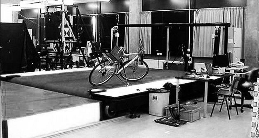
Large treadmill, 3x5 m, max speed 35 km/h, courtesy of the Faculty of Human Movement Sciences, Vrije Universiteit, Amsterdam.
The uncontrolled dynamics of the bicycle rider system can potentially be described by the linearized model of the bicycle [MPRS07]. This model consists of four rigid bodies: the rear frame with rigid rider connected, the front handlebar and fork assembly, and the two wheels. These are connected by ideal hinges and the wheels have idealized pure-rolling contact with level ground. [MKHS09] describes the method used to determine the model parameters for the instrumented bicycle-rider system[2]. These parameters are given in Table 7.3 and the root locus of the system with respect to speed is depicted in Figure 7.4. At low speed, the dominant mode is the unstable oscillatory weave mode. This weave motion becomes stable around 18 km/h, the weave critical speed. At higher speeds, the non-oscillatory capsize motion becomes unstable but since its time to double so long it is considered to be very easy to control. With those assumptions, we assert that the instrumented bicycle rider system is in need of human stabilizing control below 18 km/h and is stable otherwise.
| parameter | symbol | value for bicycle & rider |
|---|---|---|
| wheel base | \(w\) | 1.12 m |
| trail | \(c\) | 0.055 m |
| steer axis tilt (\(\pi/2\ -\) head angle) | \(\lambda\) | 0.375 rad |
| gravity | \(g\) | 9.81 N kg \(^{-1}\) |
| rear wheel radius | \(r_\mathrm{R}\) | 0.342 m |
| rear wheel mass | \(m_\mathrm{R}\) | 3.12 kg |
| rear wheel mass moments of inertia | \((I_{\mathrm{R}xx}, I_{\mathrm{R}yy})\) | (0.078, 0.156) \(\textrm{kg\ m}^2\) |
| rear body and frame mass position center of mass | \((x_\mathrm{B},\ z_\mathrm{B})\) | (0.30, -1.08) m |
| rear body and frame mass | \(m_\mathrm{B}\) | 116 kg |
| rear body and frame mass moments of inertia | \(\begin{bmatrix} I_{\mathrm{B}xx} & 0 & I_{\mathrm{B}xz}\\ 0 & I_{\mathrm{B}yy} & 0 \\ I_{\mathrm{B}xz} & 0 & I_{\mathrm{B}zz}\end{bmatrix}\) | \(\begin{bmatrix} 16.784 & 0 & -3.616\\ 0 & I_{\mathrm{B}yy} & 0 \\ -3.616 & 0 & 6.035 \end{bmatrix}\) \(\mathrm{kg\ m}^{2}\) |
| front handlebar and fork assembly position centrer of mass | \((x_\mathrm{H},\ z_\mathrm{H})\) | (0.88, -0.78) m |
| front handlebar and fork assembly mass | \(m_\mathrm{H}\) | 4.35 kg |
| front handlebar and fork assembly mass moments of inertia | \(\begin{bmatrix} I_{\mathrm{H}xx} & 0 & I_{\mathrm{H}xz}\\ 0 & I_{\mathrm{H}yy} & 0 \\ I_{\mathrm{H}xz} & 0 & I_{\mathrm{H}zz} \end{bmatrix}\) | \(\begin{bmatrix} 0.345 & 0 & -0.044\\ 0 & I_{\mathrm{H}yy} & 0\\ -0.044 & 0 & 0.065 \end{bmatrix}\) \(\mathrm{kg\ m}^{2}\) |
| Front wheel radius | \(r_\mathrm{F}\) | 0.342 m |
| Front wheel mass | \(m_\mathrm{F}\) | 2.02 kg |
| Front wheel mass moments of inertia | \((I_{\mathrm{F}xx},I_{\mathrm{F}yy})\) | (0.081, 0.162) \(\mathrm{kg\ m}^2\) |
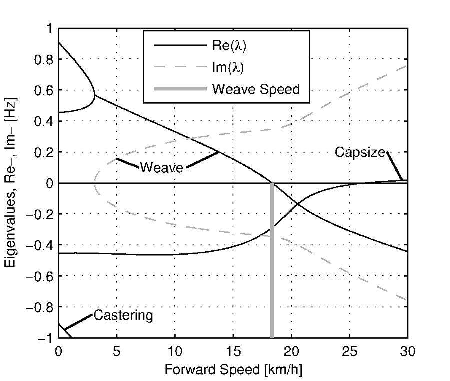
Eigenvalues for the linearized stability analysis of an uncontrolled bicycle-rider combination for the steady upright motion in the forward speed range of 0-30 km/h. Solid lines are real parts, dotted lines are imaginary parts. The bicycle is essentially stable from the weave speed, 18 km/h and above.
For safety reasons the riders were fitted with a harness that was connected to the ceiling via a long climbing rope. This ensured that should the rider fall over no contact with the moving part of the treadmill would be made. Also a retractable dog leash was connected between the front of the harness and the treadmill kill switch. This ensured that the treadmill would immediately come to a halt, should the bicycle go too far back, reducing the chance that the bicycle could go off the end of the treadmill.
Herein, three types of riding experiments are examined: normal bicycling, bicycle without pedaling (towing) and normal bicycling with lateral perturbations. The normal bicycling experiment was carried out to investigate what type of control actions a rider carries out to simply stabilize a bicycle. The towing experiment was carried out to remove the effects of the dominant pedaling motion, seen during the town-ride experiment, from the system. The bicycling with lateral perturbations was performed to investigate how the human rider recovers from a lateral impulsive force applied to the rear frame.
Each of the three experiments was carried out at 6 different speeds: 30, 25, 20, 15, 10 and 5 km/h. In total 36 experiments were performed. During the normal bicycling and bicycling with lateral perturbations experiments the rider pedalled normally and used first gear during the 5 and 10 km/h runs. Second gear was used in the 15 and 20 km/h runs and third gear was used during the 25 and 30 km/h runs. The cadence varied between 24 rpm at 5 km/h and 80 rpm at 30 km/h. During the towing series of experiments, the bicycle and rider were towed by a rope connected to the bicycle rear frame at the lower end of the head tube. The rider kept the pedals in the horizontal position during these experiments. The crank arm side that was placed forward was left to rider preference. During the lateral perturbations experiment the bicycle was perturbed by applying a lateral impulse to the rear frame. The impulse was applied by manually yanking a rope tied to the seat tube. The rider could not see the rope being actuated to ensure that the rider was unprepared, however, they knew the direction of the perturbation which was always a pull from the right.
The riders were instructed to stay on the treadmill and to generally ride in the longitudinal direction of the treadmill but not to concentrate on their exact position on the treadmill. We wanted the rider to focus on stabilization and maintaining heading and not to track lateral deviation. Sensor data was collected for 1 minute during each experiment at a 100Hz sample rate and the video data was collected simultaneously.
This video shows Arend slowly decreasing in speed. Notice the increase in steering motions as speed decreases and the little relative upper body motion at all speeds. The knees' lateral motion increases with decreasing speed also.
Normal Bicycling
Visual inspection of the video footage showed very little rider lean action during the experiment other than what resulted directly from the pedaling motion. During the low speed runs at 5 km/h, the rider’s upper body was almost stationary, i.e. it could be considered to be rigidly attached to the rear frame. However at this speed the rider’s knees showed significant lateral motion. This lateral knee motion can be seen in the video image in Figure Figure 7.5. A third observation was that the rider actuated the handlebars with higher amplitudes at lower speeds than at higher speeds.
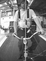
Video still of normal pedaling at low speed (5 km/h) showing large lateral (left) knee motion and (right) steering action. The grey vertical line indicates the mid-plane of the bicycle. Note that there is little upper body lean.
This third observation is confirmed by the measured steer angle data. Figures 7.6 and 7.7 show the time history of the steer angle for the experiments carried out at 20 and 5 km/h, respectively. The standard deviation of the steer angle during the sixty seconds of measurement is also shown in the figures. At speeds above 20 km/h the average steer angle remains approximately constant. However the average magnitude of the steer angle grows by more than 500% when the speed is decreased from 20 km/h to 5 km/h. This increase in steer angle magnitude for the decreasing speeds is illustrated in Figure Figure 7.8. This jump in steering amplitude could be indicative of a threshold at which the system becomes harder to control, but there is no apparent connection to the open loop dynamics. For example, the change in both the weave mode time to double and natural frequency is approximately the same between 5 and 10 km/h as between 10 and 15 km/h.
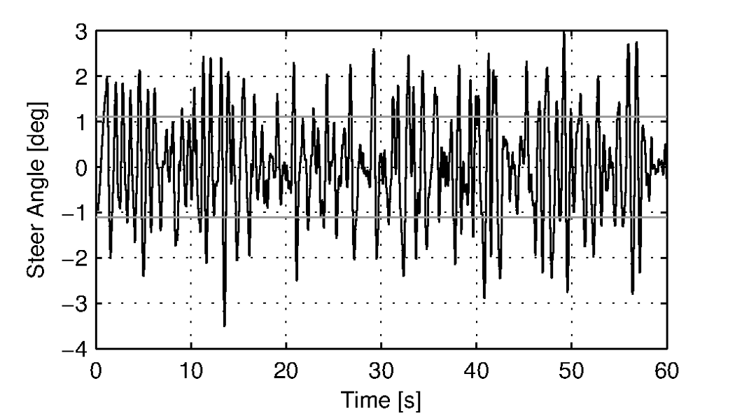
Steer angle time history plot for 20 km/h during normal bicycling. The standard deviation of the steer angle is shown in grey.
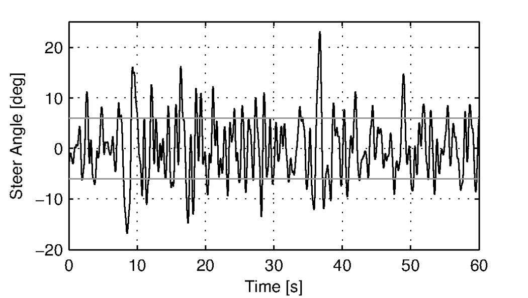
Steer angle time history plot for 5 km/h during normal bicycling. The standard deviation of the steer angle is shown in grey.
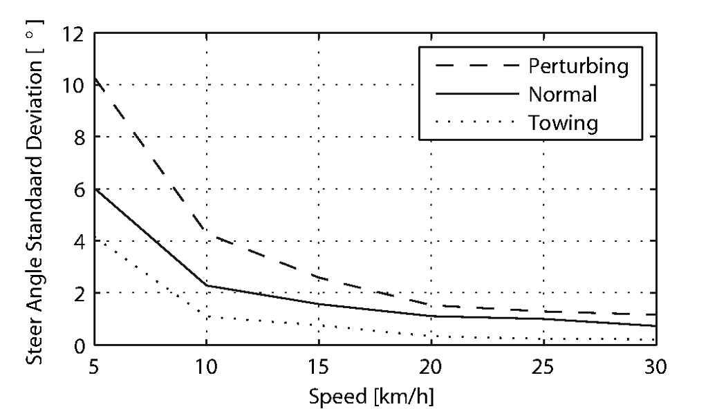
The standard deviation of the steer angle for the six different speeds for the three different experiments.
The frequency content of the steering signal for the different forward speeds is shown in Figure 7.9. The grey vertical dashed line indicates the rigid rider-bicycle weave frequency. We were not able to ascertain any connection between the dominate measured frequencies and the natural frequency of the weave mode. We had hypothesized that for speeds in the stable speed range, the optimal control frequency of the rider would correspond to the weave frequency, due to the fact that an uncontrolled bicycle-rider system recovers from perturbations at its natural frequency. The black vertical dashed line in each of the plots in Figure Figure 7.9 indicates the measured pedaling frequency. The figure shows that during normal pedaling most of steering action takes place at, or around, the pedaling frequency, irrespective of the speed that the bicycle is moving. The pedaling frequency is especially dominant in the steering signal at the highest speeds where practically all of the steering takes place at the pedaling frequency.
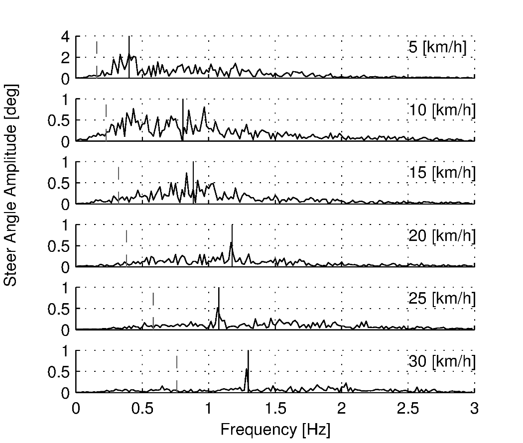
Steer angle amplitude plot for the six different speeds for normal pedaling experiment. Solid vertical line indicates the pedaling frequency. Dashed vertical grey line indicates the bicycle & rigid rider weave eigenfrequency.
Figure 7.10 plots the maximum steering amplitude versus speed. This maximum amplitude reduces with increasing speed and is similar in shape to the standard deviation plot in Figure 7.8.
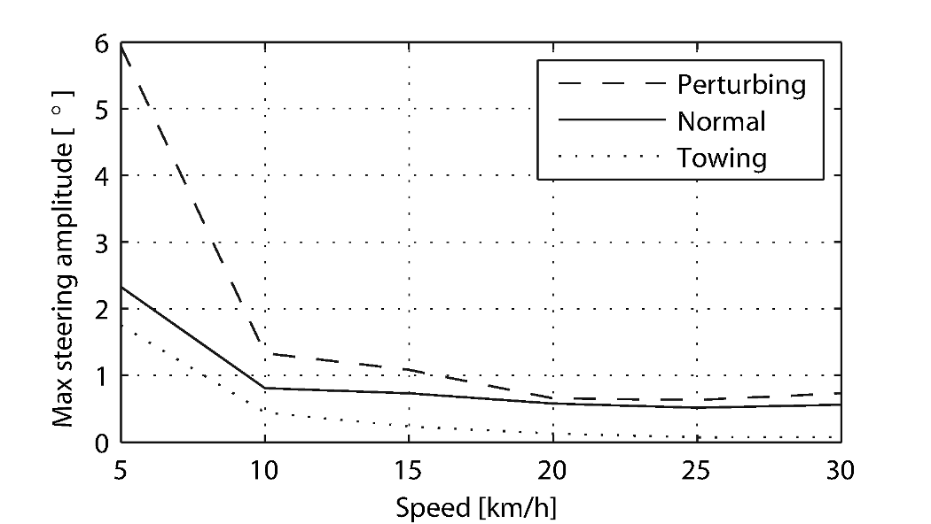
Maximum steering amplitude if the steering signal consisted of a single frequency for the three different experiments at the six different speeds.
Towing; no pedaling
Visual inspection of the video footage revealed, similar to the normal bicycling experiment, that little to no upper body leaning occurred at any of the measured speeds and that larger steer angles occurred at the slower speeds. However, unlike the normal bicycling experiment, no knee motion was noticed from visual inspection of the video footage at any of the speeds, other than small remnant motion as a result of slight steering deviations from straight ahead. The recorded steer angle data also confirmed that larger steer angles were made at decreasing speeds. Figure 7.8 shows how the standard deviation of the steer angle reduces rapidly with increasing speed up to 20 km/h and from then on remains approximately constant. The figure also shows that the average steering amplitude at all speeds is lower than that for the pedaling case. The standard deviation is less than a degree for all speeds above 10km/h indicating that little to no steer action is required at higher speeds.
The steer angle frequency spectrum for each of the speeds is shown in Figure 7.11. It was once again expected that the rigid rider/bicycle weave frequency would be a dominant frequency in the frequency spectrum, especially with no pedaling. However there appears to be no connection with the open loop weave frequency even in the unstable speed range. In fact the frequency spectrum shows a wide range of frequencies of similar amplitude at all the speeds and none of the speeds seem to show any noticeable dominant frequencies.
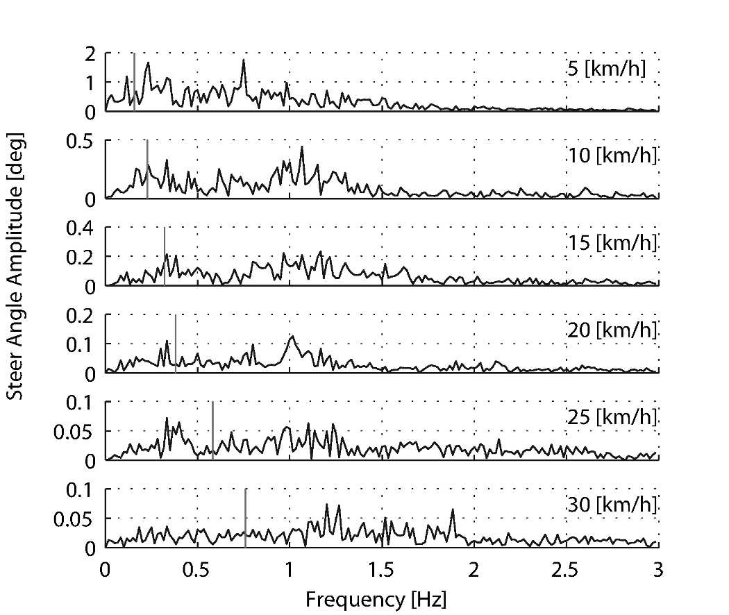
Steer angle amplitude plot for the six different speeds for the towing experiment. Vertical line indicates the bicycle & rigid rider eigenfrequency.
Perturbing; pedaling
The video footage showed that, as a result of the lateral perturbation, the bicycle was pulled laterally away from under the rider causing the bicycle to lean over and in turn cause a short transient lean motion of the rider’s upper body. The upper body appears to only lag behind the lower body and bicycle during this destabilizing part of the perturbation maneuver. During the subsequent recovery of the bicycle to the upright, straight ahead position, no body lean could be noted other than that as a result of the normal pedaling.
A second phenomenon observable in the video footage, as shown in Figure 7.12, is that at all speeds we observed a lateral knee motion during the short transient recovery process of the bicycle to the upright position. The lateral knee motion was very large during the 5 km/h measurement and much smaller at the higher speeds, but even at 30 km/h it is visible.

Video still directly after a perturbation (lateral force applied from the rider’s right by a rope at the saddle tube) at 5 km/h. Vertical grey line indicates the bicycle mid-plane. Note the lateral right knee motion and steering action and the small upper body lean.
From the video footage we also concluded that the angle that the handlebars are turned during and after a perturbation decreased with increasing speed as can also be seen in the measured steer angle data as shown in Figure 7.8.
Figure 7.13 shows the frequency spectrum of the measured steer angle. Once again, for the higher speeds, the steer control action is carried out at the pedaling frequency. At the lower speeds (5 - 10 km/h) a wider frequency range is again present but the pedaling frequency is dominant. Figure 7.10 shows the steering amplitude for the frequency with the maximum amplitude. Again the values for the highest speeds are similar to those of the standard deviation of the steer angle.
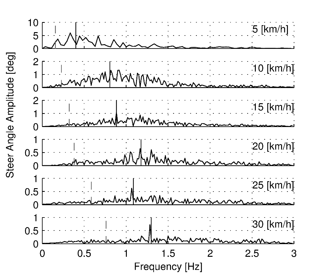
Steer angle amplitude plot for the six different speeds for perturbation experiment. Solid vertical line indicates the pedaling frequency. Dashed vertical grey line indicates the bicycle & rigid rider eigenfrequency.
Once again, the frequency spectrum shows no significant steering motion taking place at the rigid rider-bicycle weave natural frequency for any of the speeds.
Conclusion
The observations show that human stabilization control of the lateral motions of a bicycle during normal bicycling show little use of upper body lean, and that the primary control actions done through steering control. Only at very low forward speed is a potential second control action observed: knee movement. Moreover, this lateral knee motion seems to only occur while pedaling. The steering actions are dominated by the pedaling frequency while the amplitude of the steering motion increases rapidly with decreasing forward speed.
Appendix
The following sections details some extra information that was not conveyed in the papers [KS08], [KS09] and the modified version in the previous sections.
Experiments
As usual with the data deluge, we analyzed very little of the data. We recorded a total of 109 one-minute runs with two different riders. The previous sections detail only some analysis on runs from a single rider and did not include results from all of the experiments. As a result, the statistical significance of the presented analysis is somewhat weak. The following list details all of the experiments we performed:
- Normal pedaling at five speeds in which we started at the low speed, sped up to the highest and then sped down to the lowest giving twelve runs for each rider. (runs 1-6, 8-19, 101-106, 108-113)
- Normal pedaling starting at 5 km/h and decreasing speed until the rider could no longer balance with both riders. (runs 20, 21, 107, 114)
- Without pedaling (towed) at five speeds in which we either started at the low speed, sped up to the highest and then sped down to the lowest or did the opposite with both riders. (runs 22-27, 29-34, 115-120, 122-123, 126-131)
- Without pedaling starting at 5 km/h and decreasing speed until the rider could no longer balance with both riders. (runs 28, 121, 124, 125)
- Riderless weave stability test in which we increased the speed from 12 km/h to 25 km/h to try to detect the weave critical speed of the bicycle. We didn’t have much luck getting the bicycle to stabilize at all.
- Lateral perturbation at six speeds for each rider. (runs 132-133)
- No hand balancing with pedaling for one rider. (runs 60-71)
- Lane changes for both riders at six speeds. (runs 160-165, 80-85)
- A single attempt at riding with eyes closed at 30 km/h[3]
- Line tracking at six speeds for one rider. (runs 90-96)
There is potentially considerable amount of findings and better statistical conclusions that can be made from the data.
Rate Gyros
We mounted three rate sensors to the bicycle to collectively measure the yaw rate, \(u_3\), roll rate, \(u_4\), and the steer rate, \(u_7\). [4] We attached a rate gyro to the fork and handlebar assembly which measured the body fixed angular rate, \(u_{7s}\), about the steer axis, \(\hat{e}_3\). Another rate gyro was attached to the rear frame which measured the body-fixed angular rate, \(u_{3s}\), about the axis approximately aligned with gravity, \(s_\lambda\hat{c}_1 + c_\lambda\hat{c}_3\). Finally, a third rate gyro was mounted to measure the body fixed angular rate about a rearward pointing axis, \(-c_\lambda\hat{c}_1 - s_\lambda\hat{c}_3\).[5] The desired rates are found from the measurments with
We did not analyze any of the data from the rate sensors on the bicycle, but some fruitful conclusions could be drawn such as confirming the dependence of yaw rate on the steer and roll rates which come from the nonholonomic constraints. Heading and wheel contact points can be estimated well for these tasks, as the rider always tends to “zero” heading and the drift from the sensor signal integration is quite linear, see Chapter Davis Instrumented Bicycle for details. A fairly complete kinematic state of the bicycle can be estimated, ignoring frame pitch.
Steer sensor design
The steer sensor, a simple rotary potentiometer, was mounted with a design that is fairly universal for different bicycle designs, Figure 7.14. It offers axial adjust ability and belt tension. The pulley diameters were chosen for +/- 45 degrees of steering angle corresponding to about +/- 168 degrees of potentiometer angle. I originally designed it with a cord type belt, but it was later switched to a timing belt due to our worry about it slipping. I’m not 100% that belt slip did not occur and this could affect the data we collected. Integrating the steer rate from the rate gyros or differentiating the potentiometer steer angle and comparing the results to the other sensor is a way to check. I examined one run and did not find belt slip.
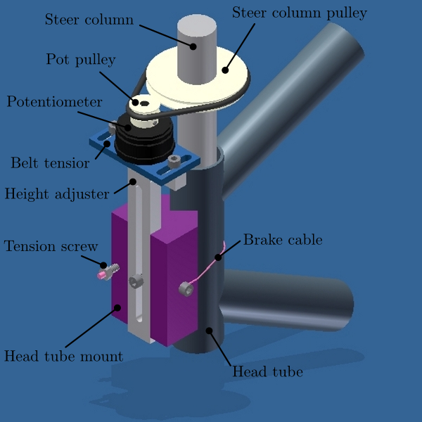
The original steer angle potentiometer and universal mount.
Data Visualization
Our original goal was to be able to visualize the motion by watching the video in slow motion or frame-by-frame along side a strip chart of the measured data. This requires some way to synchronize the video data with the sensor data. The Sony DCR-TV30E Handycam we used had a LANC output port that potentially provided an external signal that could be sampled by the data acquisition unit but we never quite figured it out. In the meantime though, I designed a graphical user interface in Matlab to interact with the data, Figure 7.15, giving the strip chart capabilities and video playback via the videoIO package developed by Gerald Dalley. All would have worked out well, if we could have synchronized the video and sensor data, but we abandoned it and moved on to other things. I’ve made the source code and data available for download in case it is of use to anyone.
- Source code: https://github.com/moorepants/DelftBicycleDataViewer
- Data: http://mae.ucdavis.edu/~biosport/DelftBicycleDataViewerAndData.zip
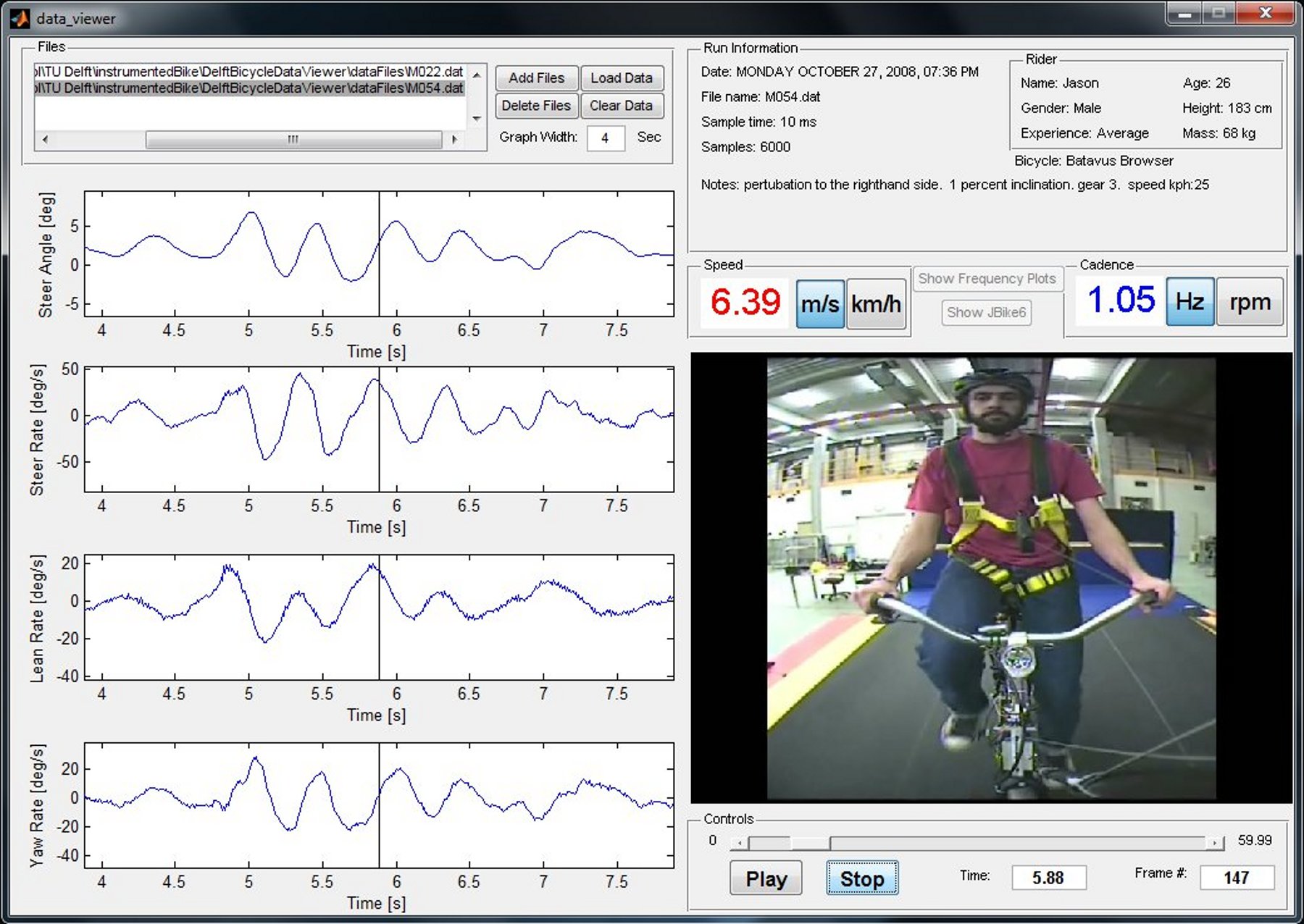
A screenshot of the GUI running on Windows 7. The strip chart advances along with the video. The user can scroll through the video and pause at select frames. The meta data for the run is displayed in the top right. The bicycle speed and the pedaling cadence are displayed as numerical values.
Rider 2
Table 7.4 presents the parameters computed with the methods in [MKHS09] for the second rider, Jason, on the instrumented Batavus Browser. Only the rear frame and body parameters are different as the bicycle is identical. We only presented data in the previous analysis from runs in which Arend rode the bicycle.
| parameter | symbol | value for bicycle & rider |
|---|---|---|
| rear body and frame mass position center of mass | \((x_\mathrm{B},\ z_\mathrm{B})\) | (0.28, -1.03) m |
| rear body and frame mass | \(m_\mathrm{B}\) | 86 kg |
| rear body and frame mass moments of inertia | \(\begin{bmatrix} I_{\mathrm{B}xx} & 0 & I_{\mathrm{B}xz}\\ 0 & I_{\mathrm{B}yy} & 0 \\ I_{\mathrm{B}xz} & 0 & I_{\mathrm{B}zz}\end{bmatrix}\) | \(\begin{bmatrix} 11.89 & 0 & -2.13\\ 0 & I_{\mathrm{B}yy} & 0 \\ -2.13 & 0 & 3.73 \end{bmatrix}\) \(\mathrm{kg\ m}^{2}\) |
Footnotes
| [1] | We took data for line tracking tasks also. |
| [2] | The instrumented bicyle was measured less accurately at this time than what is presented in Chapter Physical Parameters, so the parameters are slightly different. |
| [3] | The closed eye attempt would have been successful if the treadmill had been infinitely wide, but the run was cut short due to the inevitable lack of heading feedback the rider has available, causing the rider to drift to the edge of the treadmill. |
| [4] | The ratiometric sensor voltages were actually measured, but converted to angular rates in real time by applying the conversion factors provided by the manufacturer’s specification sheets. Thus, the angular rates are reported in the data sets. |
| [5] | See Chapter Bicycle Equations Of Motion for the axes definitions. |
