Introduction¶

Investigation of the effects of changes in the model parameters is a natural place to start once the various bicycle models are available. For the bicycle designer, understanding how changing parameters affects the dynamic characteristics is something of a holy grail. If connections can be drawn from model parameters to such things as handle-ability, stability, and controllability, bicycle designs could be tuned with these things mind. In the aircraft design world correlations have been drawn from open loop dynamics to handling qualities. It is highly likely that open loop dynamics can be predictors of the handling of a bicycle, but there are large differences in aircraft, ground vehicles, and bicycles. The most glaring is the size of the rider with respect to the vehicle and the fact that the rider’s biomechanics, which are not trivial, contribute to the open loop dynamics of the entire system.

The eigenmodes of the Whipple model and the stability regime are prime targets for initial parameter studies and there are many papers that deal with various aspects. An analytical view of the parameter relationships would provide the most encompassing conclusions, but the complicated form of the equations typically lead researchers to numerical studies. [VZ75] studies the effects of trail, front wheel moment of inertia, and rider position on the dynamics using Routh’s criterion and a sensitivity study. [KMP+11] refines the work in [Pap87] which makes use of a compact analytical form of the linear equations of motion and Routh’s stability criterion to analytically find instability the capsize mode. [FSR90] and [ASKL05] examine the effect on stable speed range of independently varying wheel rotational inertia and find that for their parameter values both the weave and capsize critical speeds decrease with increase in spin moment of inertia. [FSR90] also shows that as trail increases both the critical speeds and the stable speed range increases. This conclusion is counter intuitive, as some [Koo06] seem to believe that an increase in trail lowers the weave critical speed, thus making the bicycle more stable. [Ste09] examines experimentally and numerically the effects of the front end geometry (trail and headtube angle) on eigenvalues, with some similar results as [KSM08]. [TWB10] examines the derivatives of the critical speeds with respect to the benchmark parameters for a nominal parameter set. Tak’s method allows one to quickly visualize the independent parameter change which affects the stable speed range the most for a given bicycle. Other examples of parameter studies include [Sha71], [Sha94], [CDL99], and [LLLW03] among many others.

Numerical parameters studies were the first thing I did once I had a working Whipple model [MH08] and I’ve explored some other studies over the years. The following sections provide some of the results and various small findings.

Geometric Variation¶

My first curiosities about bicycle handling arose when I was designing the frame geometry of a recumbent bicycle for my undergraduate senior design project and this geometric outlook seems to be continually the main interest among bicycle enthusiasts and designers. Many bicycle designers focus on geometry as the primary design criterion for handling, in particular the head tube angle and trail, Figure 6.1. But wheelbase, front wheel diameter, frame/wheel alignment, and the rider position which is dictated by handlebar geometry are considered too. A browse through bicycle magazines and frame builder literature provide a wide range of opinions about how geometry affects the handling. For example, Tim Paterek, an expert frame builder, claims that the comfort zone for trail falls between 0.05 m and 0.065 m for most bicycles [Pat04a]. Craig Calfee is another prominent frame builder interested the effects of fork alignment on handling who wrote a small piece on bicycle geometry for the 2007 North American Handbuilt Bicycle show [Cal07]. He points out that minute misalignments in the fork geometry can cause undesirable handling. Finally, Jan Heine has written extensively in his Vintage Bicycle Quarterly about handling, with subjective and objective measures by experienced riders of the handling differences in real bicycles.

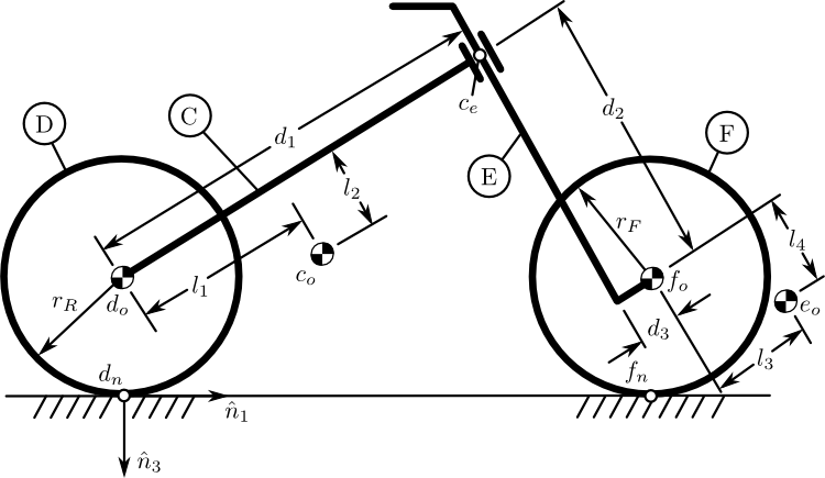
The essential geometry of a bicycle parameterized with variables typically of interest to bicycle designers.

But the reality is that little progress has been made to predict handling qualities from geometry using rigorous dynamic and control theory. Nonetheless parameter studies can still be done with the models we have available. The following results show how the stable speed range of the Whipple model linearized about the nominal configuration changes with respect to varying the essential geometry: trail, head tube angle, wheelbase, and front wheel diameter. Unlike in many other parameter studies, the physical changes associated with the rider’s position and the bicycle’s parameters other than the essential geometry are interdependent (e.g. adjusting the front wheel diameter changes the wheel’s mass and moments of inertia together with the bicycle’s frame geometry and adjusting the wheelbase causes the rider to reach further forward). It is important to point out that the parameter value combinations that result from independently varying the physical parameters do not necessarily equate to a realizable bicycle. For example, a wheel’s spin moment of inertia is generally about two times the transverse moment of inertia, so varying those parameters independently is not that useful. The rider parameters are estimated using a method which was a slight precursor to the simple geometry method presented in Chapter Physical Parameters[1] and where based off of a 72 kg, 182 cm tall adult male. The rear frame and fork were modelled as a collection of uniform steel tubes and the wheels as simple tori. This allowed estimation of the inertial properties of a bicycle as a function of geometry. It assumed a normal diamond frame bicycle and the base geometry of the bicycle was measured from a 58 cm 1982 Schwinn LeTour steel road bike.

The stable speed range for the nominal configuration was between about 3.59 m/s and 4.88 m/s. Changes in the stable speed range were calculated by varying each parameter over a realistic range for a bicycle of this nature. Each figure shows a depiction of the maximal and minimal geometry configurations and the nominal stable speed range is shown with a vertical line.

At speeds greater than the capsize critical speed, the capsize mode is unstable with a slow time to double. Thus the instability can be assumed to be relatively easy to stabilize with a simple control, especially since the weave mode provides rapid roll damping. That implies that the stable speed range and capsize critical speed may be of less importance to actual stability, leaving the weave critical speed as the defining characteristic.

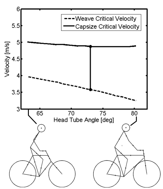
The change in stable speed range as a function of head tube angle.

A slack head tube angle (< 72 degrees) has a higher weave critical speed than a larger head tube angle but the capsize critical speed varies very little with changing head tube angle, Figure 6.2. Slack head tube angles are found on many utility bicycles. I’ve observed from experience that these bicycles feel very unresponsive at low speeds and typically do not feel stable until moderate speeds are reached. The head tube angle results, Figure 6.2 are in agreement with this anecdotal evidence insofar as the weave critical speed increases with decreasing head tube angle. The head tube angle results are interesting because the weave speed can be decreased using a steeper head tube angle without adversely affecting the capsize critical speed, thus simultaneously increasing the stable speed range and decreasing the weave speed. This is ideal if it is assumed that a low weave critical speed is beneficial for take off and a broad stable speed range is beneficial for cruising with little control input.

The change in stable speed range as a function of trail.

Trail is of particular interest, with many bicycle designers claiming that it is the most important parameter affecting handling qualities. As trail increases, the stable speed range broadens and the weave critical velocity increases, Figure 6.3. As trail approaches zero the stable speed range diminishes to zero. It is obvious that increasing trail will decrease the caster mode eigenvalue, but un-intuitively it increases the weave eigenvalue. The yellow bicycle and the silver bicycle [Koo06] both have their forks flipped for increase trail with the intent to make the bicycles stable at the speeds tested. According to the these results it does not seem that that is the case; it may have the opposite effect.

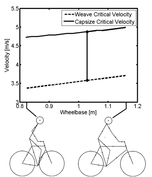
The change in stable speed range as a function of wheelbase.

Long bicycles such as tandems and some recumbents are often hard to start and have slower response due to the diminished yaw control authority. As wheelbase increases, the size of the stable speed range stays roughly constant as both weave and capsize critical speeds increase linearly at the same rate, Figure 6.4. The weave critical speed increases as wheelbase increases which correlates with the difficulty in starting long wheelbase bicycles.

The change in stable speed range as a function of front wheel diameter.

The weave critical speed decreases as front wheel diameter increases but the capsize critical speed decreases even faster so the size of the stable speed range also decreases, Figure 6.5. The results show that the weave critical speed decreases with a larger front wheel which provides stability at low speeds. This correlates with the findings for the flywheel bicycle presented in Chapter Extensions of the Whipple Model.

Here were presented some conclusions about the stability of the Whipple model and made the potential relationship of the critical speeds to geometry changes. This gives some idea of how one may begin connecting handling to the bicycle’s dynamics.

Bicycle Comparison¶

I present the physical parameters of eleven bicycles in Chapter Physical Parameters. There is a variety of bicycles from commuter bicycles to road racing and mountain to a child’s bicycle and some instrumented bicycles. Here I will present some comparisons of the linear dynamics of the different bicycles and try to make some conclusions about their dynamics. The “normal” diamond frame bicycle is very similar from bicycle to bicycle with very little variation in the essential geometry. More variation is seen in the mass and inertia.

Benchmark validity¶

The numerical values of the benchmark bicycle parameters in [MPRS07] are representative of a real bicycle but were chosen so that each parameter was guaranteed a detectable role in numerical studies. Figure Figure 6.6 compares the eigenvalues of the benchmark bicycle with those of two ordinary bicycles, the Batavus Browser and Batavus Stratos including the same rider, Jason, seated on both bicycles. The eigenvalues are qualitatively similar, but the stable speed range of the benchmark bicycle is both lower and narrower than the other two. The benchmark weave frequency also diverts from the real bicycles at higher speeds, but other than that the benchmark parameters are most likely within realistic bounds for a normal style bicycle due to the similar dynamic behavior.

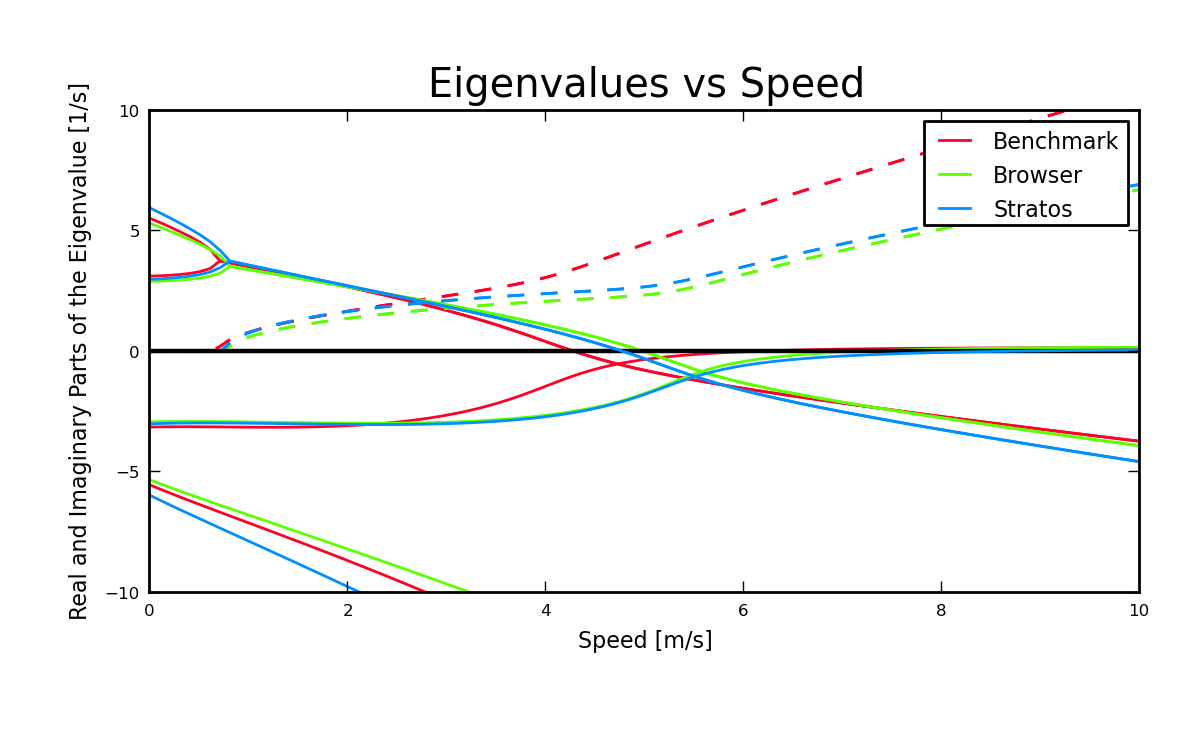
Real and imaginary parts of the eigenvalues as a function of speed for three bicycles including the benchmark bicycle from [MPRS07] and two bicycles (Browser and Stratos) and a rider (Jason) presented in Chapter Physical Parameters. Generated by src/parameterstudy/bicycle_eig_compare.py.

Rider-less bicycles¶

There are relatively few bicycles whose parameters have been measured exhaustively and accurately. Figure 6.7 plots the effect of speed on the resulting eigenvalues of one such parameter set, labeled Silver, from [KSM08] and compares it to several of the rider-less bicycles I measured using almost identical techniques to Kooijman. Notice that all of the bicycles measured in Chapter Physical Parameters show a bifurcation in the caster and capsize modes at lower speeds which produces a second oscillatory mode. This bifurcation is not necessarily seen in the parameter sets with a rigid rider. Figures 6.8 and 6.9 show the eigenvector components for the two oscillatory modes for the Crescendo bicycle at 1.5 m/s. They turn out to be similar in that they are oscillatory in roll and steer, with steer being dominant in magnitude and the phase shifts are slightly larger for the weave mode. But the new mode is stable as opposed to the weave mode being unstable. The bicycles measured in [Ste09] and [ER11] both exhibit this mode, but Stevens’ [Ste09] parameters are estimated from a CAD drawing, which may not be as accurate as more direct measurements. Steven’s does show that this mode disappears with very steep or very slack head tube angles. The diagrams for very slack head angles more qualitatively resemble the Silver bicycle from [KSM08]. But it is still odd that the Silver bicycle is that different than all the other bicycles, with the only major difference being a flipped fork for more trail and a larger yaw and roll moment of inertia due to the outriggers.

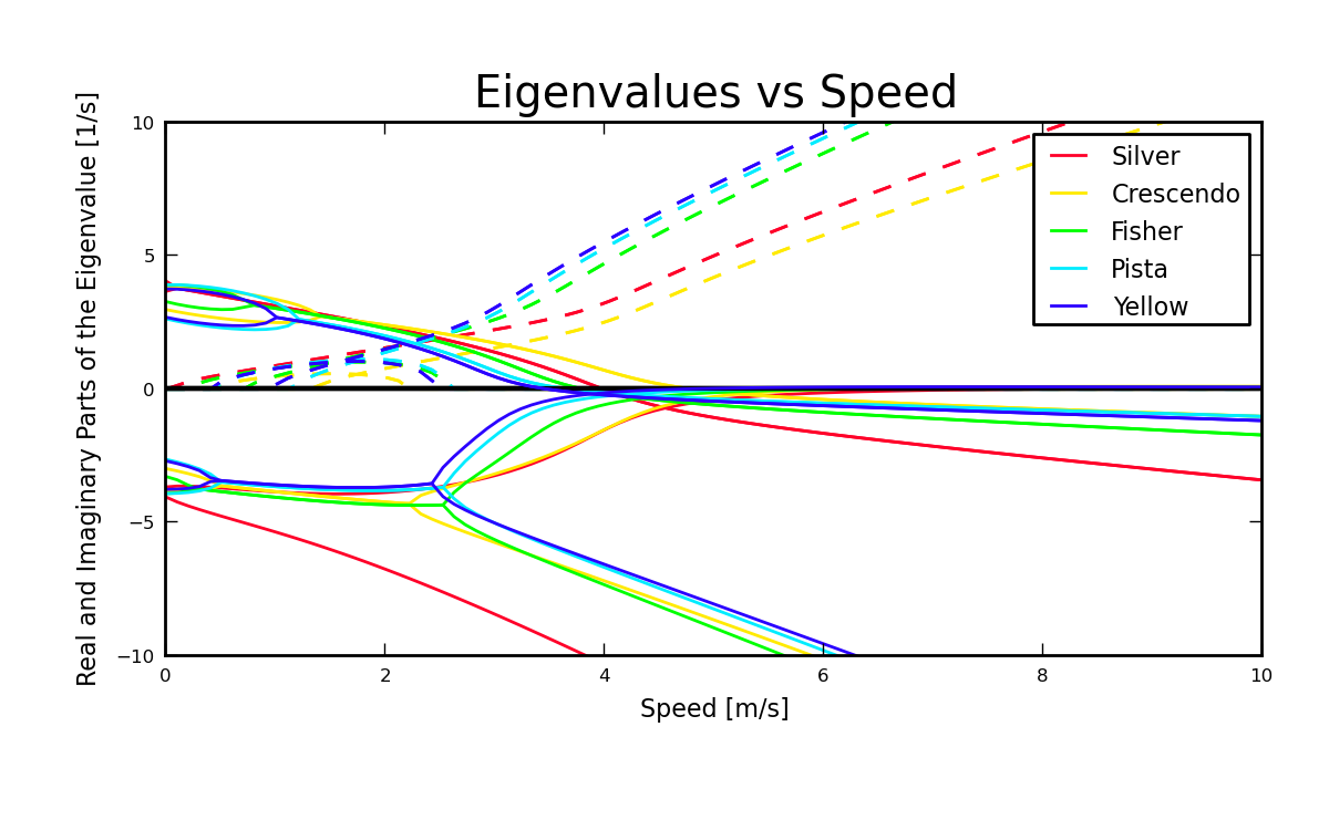
Real and imaginary parts of the eigenvalues as a function of speed for four bicycles including the silver bicycle from [KSM08] and three bicycles and riders presented in Chapter Physical Parameters. Generated by src/parameterstudy/bicycle_eig_compare.py.

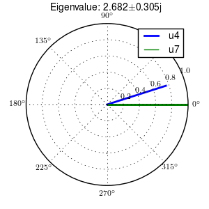
Eigenvector components for roll rate, \(u_4\), and steer rate, \(u_9\), for the Crescendo parameter values weave mode at 1.5 m/s. Generated by src/parameterstudy/bicycle_eig_compare.py.

Eigenvector components for roll rate, \(u_4\), and steer rate, \(u_9\), for the Crescendo parameter values new mode at 1.5 m/s. Generated by src/parameterstudy/bicycle_eig_compare.py.

Bicycles with riders¶

There are some potentially significant differences in the Whipple model dynamics between a riderless bicycle and a bicycle with a rider. Figure 6.10 gives an example of how the eigenvalues change when a rider is added to the Stratos bicycle. The stable speed range broadens and the weave critical speed increases by more than 1 m/s. The second oscillatory mode disappears and the caster decays more rapidly. The weave bifurcation occurs at a lower speed. And finally the natural frequency of the weave mode for the rider and bike is much lower for speeds above 3 m/s. The changes in dynamics are large enough that conclusions made about bicycles without rigid riders don’t necessarily extend to bicycles with rigid riders.

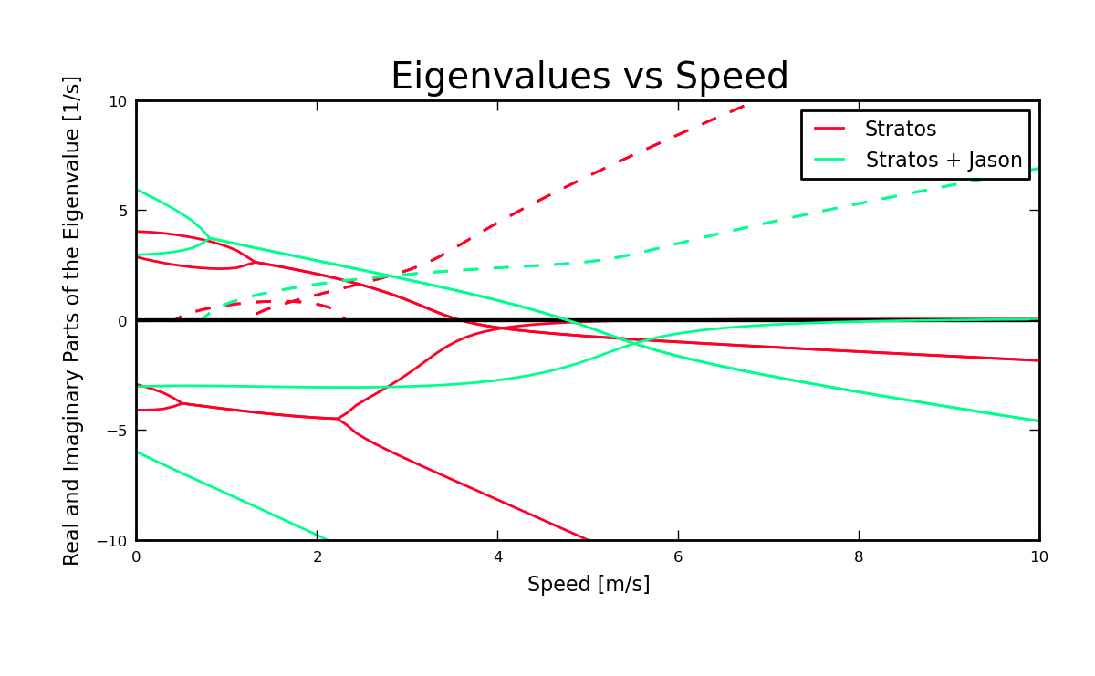
Real and imaginary parts of the eigenvalues with respect to speed for the Stratos bicycle with and without a rider. Generated by src/parameterstudy/bicycle_eig_compare.py.

Yellow bicycle¶

I measured the parameters of the “Yellow” bicycle at TU Delft, which was a replica of the Yellow bike from Cornell that demonstrates stability so well. I measured the bicycle in two configurations, one with the fork in the normal position and the second with the fork flipped 180 degrees about the steer axis which greatly increases trail. Figure 6.11 plots the eigenvalues with respect to speed for the two yellow bicycle configurations and the Silver bicycle [KSM08] which also has a reversed fork and large trail. As was mentioned in the previous section the weave critical speed increases as the trail increases and this is clearly shown for the yellow bicycle with a reversed fork. But maybe more interestingly, the capsize critical speed increases dramatically with the reversed fork.

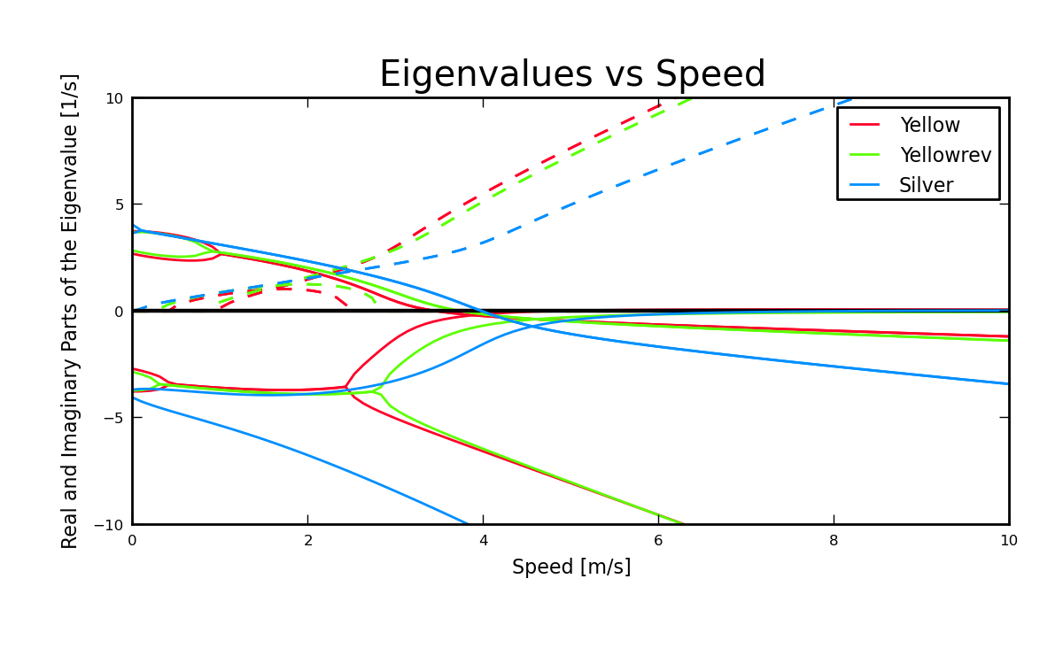
Real and imaginary parts of the eigenvalues respect to forward speed for the yellow bicycle in both configurations and the silver bicycle which also has a reversed fork. Generated by src/parameterstudy/bicycle_eig_compare.py.

The classic yellow bicycle stability demonstration from Cornell University.

Rear weight¶

Another fruitful comparison can be gathered from the Batavus Browser as we measured both the instrumented configuration and the factory version. The fundamental difference in the two configurations is that the instrumented version has a large weight atop the rear rack. Bicycle tourists are some of the first to mention the effects on handling due to weight on the front and rear racks of a bicycle, so this comparison examines that to some degree. Figure 6.12 once again shows how the eigenvalues change with respect to speed for the two bicycles. The second bifurcation points for the second oscillatory mode are affected and the weave critical speed is slightly lower for the factory version. If a rider is added, Figure 6.13, shows that the added rear weight makes little difference in the linear dynamics.

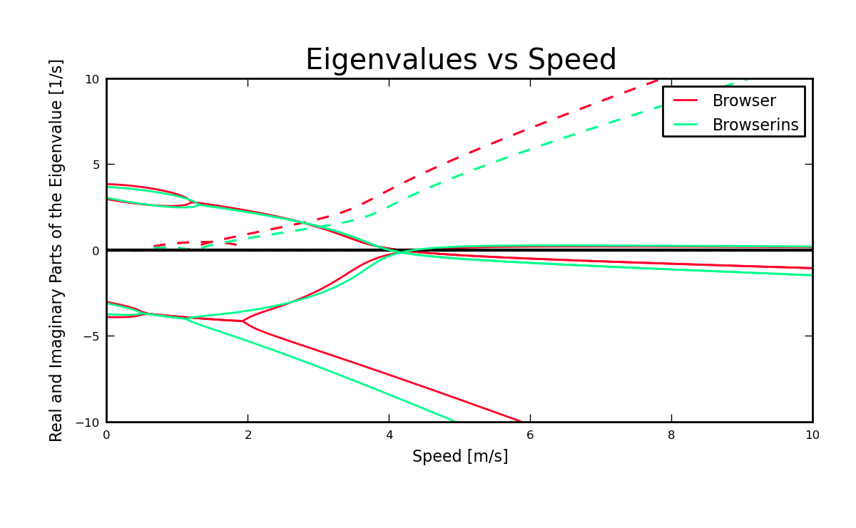
Real and imaginary parts of the eigenvalues with respect to forward speed for the factory Browser and the instrumented version which has a large weight on the rear rack. Generated by src/parameterstudy/bicycle_eig_compare.py.

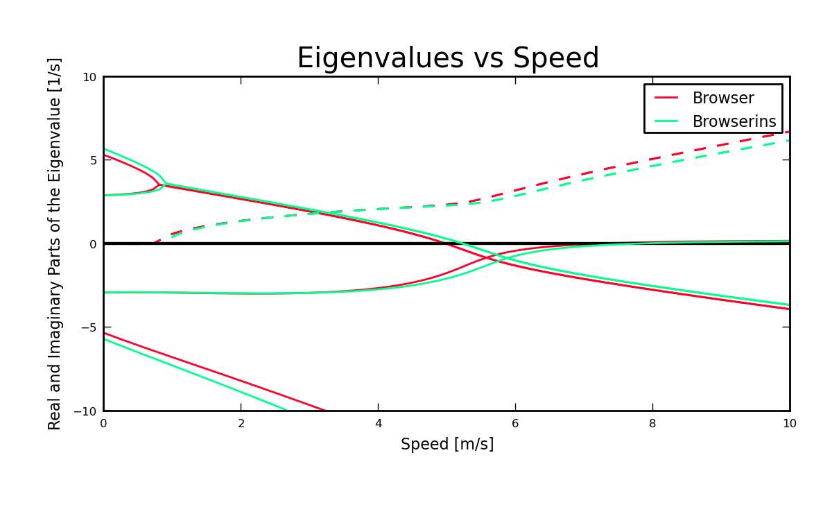
Real and imaginary parts of the eigenvalues with respect to forward speed for the factory Browser and the instrumented version which has a large weight on the rear rack and a rider. Generated by src/parameterstudy/bicycle_eig_compare.py.

Uncertainty¶

I had intended to calculate the uncertainty in the eigenvalue predictions based on the error propagation from the raw measurements, but I never quite figured it out. It would be interesting to draw error bars on the modes in the eigenvalue plots corresponding to the uncertainty values presented in Chapter Physical Parameters. It would be revealing with respect to the experiments that are done which try to estimate the eigenvalues of a stable bicycle [KSM08], [KS09], [Ste09], [ER10]. All of the these experiments, except for [KS09], plot a predicted eigenvalue for a speed range because it is difficult to maintain constant speed with an uncontrolled bicycle, but beyond that the uncertainty in the eigenvalue estimates is not reported. These could also be calculated with respect to the fit data. It would be interesting to account for the uncertainties in both methods of predicting the eigenvalues and then compare the model’s ability to predict the data. Because the eigenvalues seem to be rather sensitive to changes in some parameters, this may be an important issue to address.

Frequency Response¶

The eigenvalues give a complete view of the linear system’s open loop dynamics, but one can also examine the system’s response to various inputs. The frequency response characterizes how the system responds to a sinusoidal input.

The transfer function from steer torque to the roll rate of a bicycle is particularly interesting because it captures the essential steering action needed to induce a turn. Figure 6.14 shows the transfer function for Jason seated on the Browser for several different speeds. The speeds correspond to before the first weave bifurcation, unstable weave, stable speed range and unstable capsize. The roll rate amplitudes increase somewhat with speed, with the 6 m/s case showing larger output amplitudes than the more well damped 10 m/s one. The phase shows similarity between the higher two speeds and similarity between the lower two speeds where the phase is roughly the same for all speeds at high frequency. Both the magnitude and phase show differences at lower frequencies and seem to tend to the same response at higher frequencies.

The steer torque to roll rate frequency response for various speeds.

Figure 6.15 shows the transfer function for the same rider (same configuration with respect to the rear wheel contact point) seated on a light weight bicycle, the Bianchi Pista, and very heavy bicycle, the Davis instrumented bicycle. Notice that the light bicycle has an under-damped weave mode which is stable, while the heavy bikes weave mode is well damped and unstable. Once again, differences in the frequency response are less apparent at high frequencies.

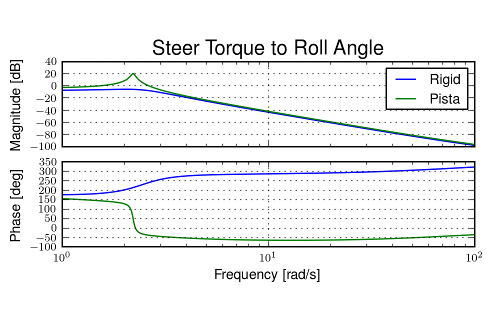
The steer torque to roll rate frequency response for a heavy and light bicycle, both with riders, at 5 m/s.

Conclusions¶

Parameter studies can allow one to explore the effects of design parameters on the system dynamics of particular bicycles. The eigenvalues provide a way to transform the parameters of a complex system into a minimum characteristic set of parameters that completely characterize the open loop (input ignorant) dynamics. And other characterizations such as the frequency response provide input/output behavior of the system’s transfer functions. System stability, time to double/halve, natural frequency, and frequency responses are all important characteristics of the system. There are likely to be correlations from the open loop dynamics to handling, as has been demonstrated in the aircraft control literature, but currently correlations to bicycle handling are mostly speculative and anecdotal at this point.

For a basic diamond frame bicycle, large changes in parameters seem to be needed for large changes in the dynamics. Most bicycle design parameter values are such that the dynamic behavior is quite similar across designs and their differences may not be readily detectable by the human. [TWB10] shows that changes in only a few parameters can make a large difference in the stable speed range of the benchmark bicycle. Even if these changes are detectable by the rider, they are extremely adaptable to minor bicycle design variations in terms of the ability maneuver the bicycle, i.e. it takes little time to become comfortable with a different bicycle. This seems evident even with regards to changes in the front end geometry such as trail; countless debates have ensued over the effect of this parameter. Negative trail recumbents have been designed and the rider can learn to ride them, but they require a higher learning curve, see the Python Lowracer [Mag12] for an example. These bikes are difficult to learn but with practice they often be easily ridden with no hands. With this in mind, the open loop dynamics of most standard diamond frame bicycles don’t really vary much, but this surely doesn’t include tandems, large two wheel cargo bicycles, recumbent designs, etc. I’ve also shown that the differences in dynamics between a riderless bicycle one with a rigid rider can be significant. Parameter studies may let us find bicycle designs that don’t fit the normal mold but may still have good handling, see [KMP+11] for some examples of exploring the extremes of the parameter space.

I’ve shown some qualitative comparisons for real and realistic bicycles. It is highly likely that the open loop weave eigenvalue and the critical speed (if there is one) correlate to what a rider feels when riding a bicycle, but this has yet to be proven with strong experimental evidence. Everyone can agree that balance is more difficult when starting up than at cruising speed. The dynamics show that the system becomes more stable and more controllable (in the control system sense) as the speed increases. The weave eigenvalue and critical speed are currently as good indicators of stability one can get for normal bicycle designs.

Footnotes