We will use the same differential equations for the SIR model as previously introduced. The right hand side of the ordinary differential equations are evaluated with the following function eval_SIR_rhs.m:
function xdot = eval_SIR_rhs(t, x, c)
  % Inputs:
  % t : 1x1 scalar time
  % x : 3x1 state vector [S; I; R]
  % c : structure containing 2 constant parameters
  % Outputs:
  % xdot : 3x1 state derivative vector [S'; I', R']

  S = x(1); % susceptible [person]
  I = x(2); % infected [person]
  R = x(3); % recovered [person]

  beta = c.beta;  % infectious contacts per time [person/day]
  tau = c.tau;  % mean infectious period [day]

  N = S + I + R;

  Sdot = -beta*I*S/N;

  Idot = beta*I*S/N - I/tau;

  Rdot = I/tau;

  xdot = [Sdot; Idot; Rdot];

end
The following function euler_integrate.m implements Euler's Method of integration and is designed to be a drop in replacement for ode45():
function [ts, xs] = euler_integrate(f, ts, x0)
% f: function handle for the state derivative function
% ts: 1xn vector of time values
% x0: mx1 vector of initial states
% xs: nxm matrix where each column is the state at the ith time

xs = zeros(length(ts), length(x0));  % nxm matrix of zeros

xs(1, :) = x0;  % set first row to initial condition

for i=2:length(ts)
    deltat = ts(i) - ts(i - 1);
    % note the transpose ' operators to ensure the dimensions match,
    % as xs(i - 1, :) is 1xm instead of mx1
    xs(i, :) = xs(i - 1, :)' + deltat * f(ts(i - 1), xs(i - 1, :)');
end

end
The ordinary differential equations are integrated (simulated) with the following script simulate_SIR_model_euler.m:
% constant parameters
c.beta = 1/7;  % infectious contacts per day [person/days]
c.tau = 14;  % days infectious [day]

% intial population values
S0 = 39.56E6;  % population of California [person]
I0 = 1000;  % infected [person]
R0 = 200;  % recovered [person]

x0 = [S0; I0; R0];

num_months = 8;
num_days_per_month = 30;

ts = 0:num_months*num_days_per_month;  % units of days

% integrate the equations with both the Euler method and ode45 (Runga-Kutta
% method)
f = @(t, x) eval_SIR_rhs(t, x, c);
[ts, xs] = euler_integrate(f, ts, x0);

[ts2, xs2] = ode45(f, ts, x0);

% plot the results, comparing the two integration results
hold on
title(sprintf('R0 = %1.2f', c.beta*c.tau))
plot(ts, xs(:, 1), 'b', ts2, xs2(:, 1), 'b--')  % S(t)
plot(ts, xs(:, 2), 'r', ts2, xs2(:, 2), 'r--')  % I(t)
plot(ts, xs(:, 3), 'g', ts2, xs2(:, 3), 'g--')  % R(t)
xlabel('Time [days]')
ylabel('Number of people')
legend('S (Euler)', 'S (ode45)', ...
       'I (Euler)', 'I (ode45)', ...
       'R (Euler)', 'R (ode45)')
hold off
And produces the following figure:
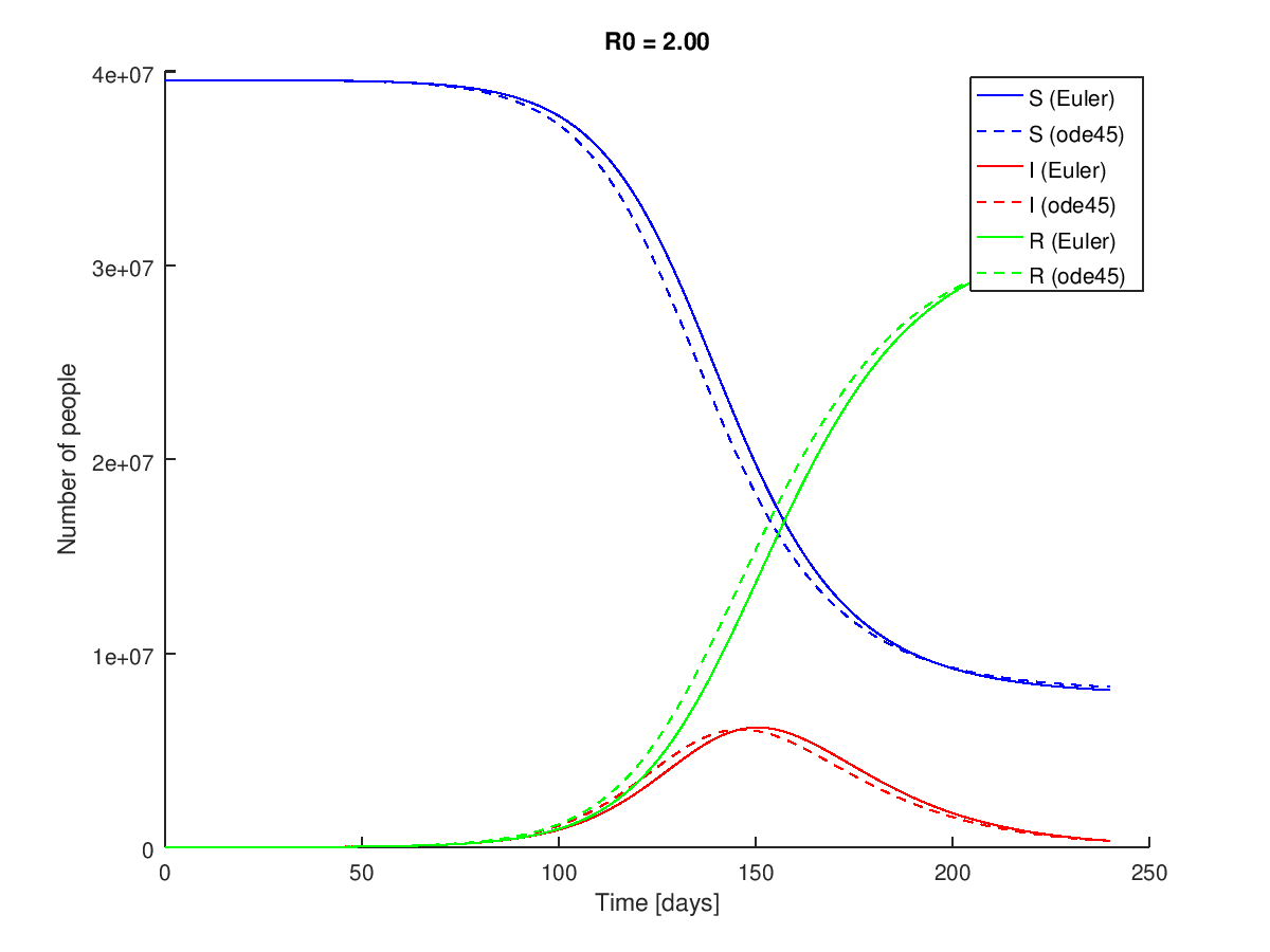
The Euler Method deviates from the ode45() solution due to the poorer error properties of the method.
The following was not covered in lab, but you may find it interesting.
A simple Runga-Kutta Method of order 4 can also be implemented and compared to the Runga-Kutta method used by ode45(). The file runga_kutta_integrate.m is shown below:
function [t, x] = runga_kutta_integrate(f, t, x0)
    % RUNGA_KUTTA_INTEGRATE - Integrates a set of first order ordinary
    % differential equations using the 4th order Runga-Kutta method.
    %
    % Syntax: [t, x] = runga_kutta_integrate(f, t, x0)
    %
    % Inputs:
    %   f - An anonymous function that evaluates the right hand side of the
    %       first order ordinary differential equations, i.e. dx/dt. The
    %       function must follow the syntax dxdt = f(t, x) and return a size
    %       mx1 vector where t is size 1x1 and x is size mx1.
    %   t - Vector of monotonically increasing time values. [size 1xn]
    %   x0 - Vector a initial conditions for the states. [size mx1]
    % Outputs:
    %   t - Vector of monotonically increasing time values (same as the
    %       input t). [size 1xn]
    %   x - Matrix of state values as a function of time. [size nxm]

    % Create an "empty" matrix to hold the results n x m.
    x = nan * ones(length(t), length(x0));

    % Set the initial conditions to the first element.
    x(1, :) = x0;

    % Use a for loop to sequentially calculate each new x.
    for i = 2:length(t)
        deltat = t(i) - t(i-1);

        k1 = f(t(i - 1), x(i - 1, :)');
        k2 = f(t(i - 1) + deltat/2, x(i - 1, :)' + deltat.*k1./2);
        k3 = f(t(i - 1) + deltat/2, x(i - 1, :)' + deltat.*k2./2);
        k4 = f(t(i), x(i - 1, :)' + deltat.*k3);

        x(i, :) = x(i - 1, :)' + 1/6*deltat*(k1 + 2*k2 + 2*k3 + k4);

    end

end
The ordinary differential equations are integrated (simulated) with the following script simulate_SIR_model_ode45_euler.m:
% constant parameters
c.beta = 1/7;  % infectious contacts per day [person/days]
c.tau = 14;  % days infectious [day]

% initial population values
S0 = 39.56E6;  % population of California [person]
I0 = 1000;  % infected [person]
R0 = 200;  % recovered [person]

x0 = [S0; I0; R0];

num_months = 8;
num_days_per_month = 30;

ts = 0:num_months*num_days_per_month;  % units of days

% integrate the equations
f = @(t, x) eval_SIR_rhs(t, x, c);
[ts, xs] = ode45(f, ts, x0);

[ts2, xs2] = euler_integrate(f, ts, x0);

[ts3, xs3] = runga_kutta_integrate(f, ts, x0);

% plot the results
hold on
title(sprintf('R0 = %1.2f', c.beta*c.tau))
plot(ts, xs(:, 1), 'b', ts2, xs2(:, 1), 'b--', ts3, xs3(:, 1), 'b.')  % S(t)
plot(ts, xs(:, 2), 'r', ts2, xs2(:, 2), 'r--', ts3, xs3(:, 2), 'r.')  % I(t)
plot(ts, xs(:, 3), 'g', ts2, xs2(:, 3), 'g--', ts3, xs3(:, 3), 'g.')  % R(t)
xlabel('Time [days]')
ylabel('Number of people')
legend('Susceptible (ode45)', 'Susceptible (Euler)', 'Susceptible (RK)', ...
       'Infected (ode45)', 'Infected (Euler)', 'Infected (RK)', ...
       'Recovered (ode45)', 'Recovered (Euler)', 'Recovered (RK)')
hold off
And produces the following figure:
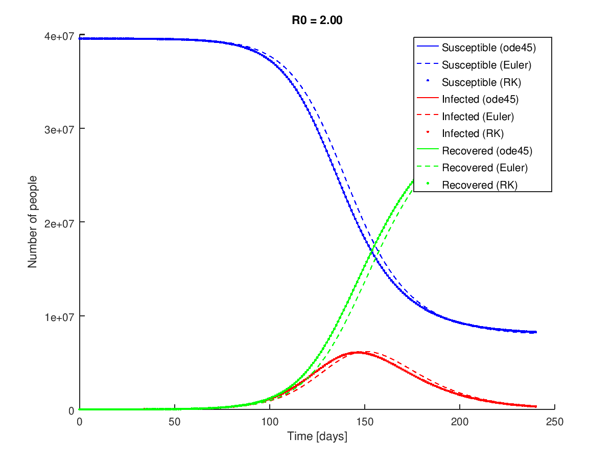
The custom Runga-Kutta method is essentially identical to the ode45() result for this system.