Contents
Learning Objectives
After completing this lab you will be able to:
- translate ordinary differential equations into a computer function that evaluates the equations at any given point in time
- numerically integrate ordinary differential equations with Octave/Matlab's ode45
- create complete and legible plots of the resulting input, state, and output trajectories
- create a report with textual explanations and plots of the simulation
Information
Extra information (asides) are in blue boxes.
Warnings
Warnings are in yellow boxes.
Introduction
This lab assignment deals with using engineering computation to numerically integrate the differential equations generated from modeling the dynamics of a system. The process of integrating these time dependent equations is called "simulation". Simulation is a powerful tool for studying both linear and non-linear systems. In this case, the differential equations are provided to you and your job is to translate them into correctly functioning m-files and show through plots that the simulation is working as expected and make some observations about the system's behavior. As we move forward in the course you will apply this method to other problems.
We have created a guide that explains how to create a working simulation of a simple torque driven pendulum system. Using this guide, your goal for this lab is to apply the same methods to the vehicle dynamics example problem described below.
The Example System
A train car is generally mounted atop two bogies, one fore and one aft. The fixed axle wheelsets are then mounted to the bogies. The bogies house the suspension system that isolates the train car from the wheelsets. The nature of the flexible coupling between the wheelsets and the train car as well as the dynamics of the wheelset-track interaction can cause oscillations to occur. These oscillations can even be unstable and cause derailments. The oscillations are called "Hunting Oscillation" or "truck hunting" ("truck" refers to the bogie and wheelset). Take a look at these videos to see some examples and explanations of hunting oscillations:
- Train car hunting @ 1:38 [1:51]: https://youtu.be/n-EfKFxGJc4k
- Damaged car hunting @ 1:08 [2:13]: https://youtu.be/JHT-WJWdjEk
- Several cars hunting [2:58]: https://youtu.be/3i-ViwHubeE
- Animation of train truck hunting [0:28]: https://youtu.be/5GwF6x7F1LM
- Bullet train wheel design, hunting @ 2:45 [9:34]: https://youtu.be/SRsm7mv0Oh8 (this is pretty unscientific and doesn't give precisely correct information but it has some good visuals regardless, so don't believe everything the host is saying)
Below is a schematic of a simple model of this system. This schematic is explained in detail in Chapter 10 of the course textbook, but for the purposes of this lab you will need to have a basic understanding of the geometry. The fixed axle wheelset is connected to the car by four linear springs of stiffnesses \(k_1\) and \(k_2\). The car and the center of the wheelset are moving at a constant speed \(V\). The wheelset can move laterally relative to the car and tracks. This lateral deviation is tracked by the time varying variable \(q_1\). The yaw rotation angle of the wheelset relative to the car and tracks is measured by the time varying variable \(q_2\). The wheel-track connection is modeled by concave wheel surfaces rolling on a convex track surface with radii \(R\) and \(R'\), respectively. When there is no lateral deviation and no yaw angle, \(q_1=q_2=0\), the nominal radius at the wheel-track contact location is \(r_0\) and the angle of the line tangent to the connecting surfaces is \(\delta_0\).
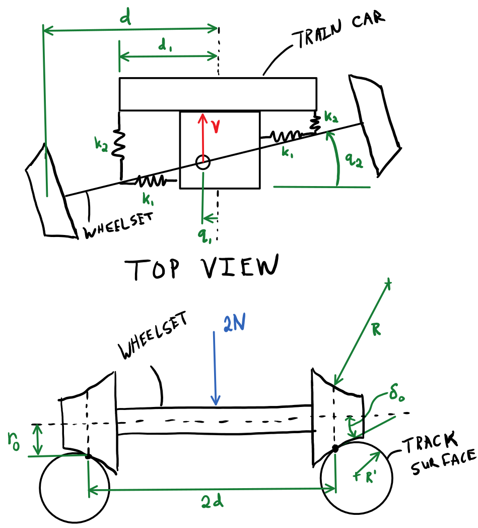
Figure 1: Schematics of the train wheelset model. See figures 10.1, 10.2, and 10.3 in the book for more detail. The upper figure is the top view and the lower figure is a rear view.
Equations of Motion
With careful attention to formulating the kinematics and dynamics, the explicit coupled first order linear ordinary differential equations that describe how the dynamics of the system change with respect to time can be found. You will learn how to generate these equations as we move forward in this class. For now, we provide you with the resulting four equations:
These equations define expressions for the derivatives of the four time varying state variables \(q_1(t),q_2(t),u_1(t),\) and \(u_2(t)\) which are described below.
| Symbol | Description | Units |
|---|---|---|
| \(q_1\) | Wheelset lateral deviation | \(\textrm{m}\) |
| \(q_2\) | Wheelset yaw angle | \(\textrm{rad}\) |
| \(u_1\) | Wheelset lateral velocity | \(\textrm{m/s}\) |
| \(u_2\) | Wheelset yaw angular velocity | \(\textrm{rad/s}\) |
You will use the section Defining the State Derivative Function for these equations.
Terminology for differential equations
- differential equation: mathematical equation that relates functions and their derivatives
- ordinary differential equation: differential equations that only have deriviatives of a single variable; in our case time is the variable
- coupled: the same time varying variables appear in more than one equation
- explicit: all the time derivatives are on the lefthand side of the equations
- linear: the derivatives are strictly linear functions of the time varying variables on the right hand side
Constant Parameters
The majority of the variables in the four differential equations above do not vary with time, i.e. they are constant. Below is a table with an explanation of each variable, its value, and its units. Note that the units are a self consistent set of SI base units.
| Symbol | Description | Value | Units |
|---|---|---|---|
| \(I_W\) | Yaw moment of inertia of the wheelset | \(m_w d^2\) | \(\textrm{kg}\cdot\textrm{m}^2\) |
| \(N\) | One quarter of the weight of the train car | \(W/4\) | \(\textrm{N}\) |
| \(R\) | Wheel surface radius | 0.23 | \(\textrm{m}\) |
| \(R'\) | Rail surface radius | 0.2 | \(\textrm{m}\) |
| \(V\) | Car longitudinal speed | 40 | \(\textrm{m/s}\) |
| \(W\) | Train car weight | 80000 | \(\textrm{N}\) |
| \(d\) | Half the track width | 0.72 | \(\textrm{m}\) |
| \(d_1\) | Distance to yaw spring | \(d/2\) | \(\textrm{m}\) |
| \(\delta_0\) | Nominal wheel-rail contact angle | \(\pi/180\) | \(\textrm{rad}\) |
| \(f_x\) | Lateral creep coefficient | \(1\times10^6\) | Unitless |
| \(f_y\) | Longitudinal creep coefficient | \(1\times10^6\) | Unitless |
| \(k_1\) | Lateral spring stiffness | 13000 | \(N/m\) |
| \(k_2\) | Longitudinal spring stiffness | 13000 | \(N/m\) |
| \(m_W\) | Wheelset mass | 1000 | \(\textrm{kg}\) |
| \(r_0\) | Nominal wheel contact radius | 0.46 | \(\textrm{m}\) |
| \(\lambda\) | Conicity | \(\frac{R\delta_0}{R - R'}\) | Unitless |
You will use the section Integrating the Equations to for these values.
Outputs
A train designer may be interested in knowing how much force is applied to the wheels at the contact location from the track so that they can size the components appropriately. The lateral and longitudinal wheel contact forces on the right wheel can be estimated by these functions:
You will use the section Outputs Other Than The States to compute these values.
Initial Conditions
Initial conditions are the starting values for the integrated state variables in the systems. This system has four state variables, so there are four initial conditions. For this lab, use the initial values shown below. See Integrating the Equations for how to set up the initial condition vector. Make sure that your initial conditions are arranged in the same order as your state variables.
Time Steps
You will also have to decide on how long your simulation will run and at what time resolution you should report values of the states, inputs, and outputs. Some rules of thumb for making these choices:
- If your system is stable and decays, choose a simulation duration such that the amplitude has decayed at least 95% of the maximum amplitude.
- If your system oscillates, show at least 5 full periodic oscillations.
- If your system oscillates, plot as least fifty time points for the shortest observed oscillation period.
Use these rules of thumb to select a simulation duration and time step spacing for your simulations.
Deliverables
In your lab report, show your work for creating and evaluating the simulation model. Include any calculations you had to do, for example those for initial conditions, input equations, time parameters, and any other parameters. Additionally, provide the indicated plots and answer the questions below. Append a copy of your Matlab/Octave code to the end of the report. The report should follow the report template and guidelines.
Submit a report as a single PDF file to Canvas by the due date that addresses the following items:
- Create a function defined in an m-file that evaluates the right hand side of the ODEs, i.e. evaluates the state derivatives. See Defining the State Derivative Function for an explanation.
- Create a function defined in an m-file that calculates the two outputs: lateral and longitudinal force at the right wheel. See Outputs Other Than the States for an explanation.
- Create a script in an m-file that utilizes the above two functions to simulate the train system. This should setup the constants, integrate the dynamics equations, and plot each state, and output versus time. See Integrating the Equations for an explanation.
- Simulate the system twice, first at V=20 m/s (72 km/h) and then at V=50 m/s (180 km/h). Plot all four state variables and the two output variables in a single subplot that has six rows, making one plot for each simulation. Use plots and written text to describe the differences in the observed motion at the two speeds.
- Set the velocity back to V=20 m/s and make the wheel surface radius \(R\) convex instead of concave by making the value negative. Plot the resulting simulation state and output trajectories in a single subplot. Describe the motion as compared to the simulation at 20 m/s with concave wheel surfaces and what you learn from it.
Use the templates below for developing your code and fill in the missing pieces.
Templates for Coding
Provided below are templates to utilize in coding the first lab. Your code should be identical to the templates, but it is your job to fill in the missing information.
Defining the State Derivative Function
function xdot = eval_train_wheelset_rhs(t, x, c)
% EVAL_TRAIN_WHEELSET_RHS - Returns the time derivative of the states, i.e.
% evaluates the right hand side of the explicit ordinary differential
% equations for the train wheelset model.
%
% Syntax: xdot = eval_train_wheelset_rhs(t, x, c)
%
% Inputs:
%   t - Scalar value of time, size 1x1.
%   x - State vector at time t, size 4x1, [q1; q2; u1; u2]
%   c - Constant parameter structure with 16 parameters.
% Outputs:
%   xdot - Time derivative of the states at time t, size 4x1.

% unpack the states into useful variable names
% replace the question marks with useful variable names
? = x(1);
? = x(2);
? = x(3);
? = x(4);

% unpack the parameters into useful variable names
% replace the question marks with your code and add all constants
? = c.?;
? = c.?;
? = c.?;

% calculate the derivatives of the state variables

replace this line of code with your lines of code

% pack the state derivatives into an mx1 vector
xdot = [q1dot; q2dot; u1dot; u2dot];

end
Defining the Output Function
function y = eval_train_wheelset_outputs(t, x, c)
% EVAL_TRAIN_WHEELSET_OUTPUTS - Returns the output vector at the specified
% time.
%
% Syntax: y = eval_train_wheelset_outputs(t, x, c)
%
% Inputs:
%   t - Scalar value of time, size 1x1.
%   x - State vector at time t, size 4x1, [q1; q2; u1; u2]
%   c - Constant parameter structure with 16 parameters.
% Outputs:
%   y - Output vector at time t, size 2x1, [Fx; Fy].

% unpack xdot and x as needed

replace this line with your lines

% unpack the parameters

replace this line with your lines

% calculate the forces

replace this line with your line(s)

% pack the outputs into a qx1 vector
y = [Fx; Fy];

end
Solving the Integration of ODEs
% define the initial conditions
x0 = ?

% define a set of time values
ts = ?

% set the numerical values for the constants
c.? = ?;
c.? = ?;
c.? = ?;
c.? = ?;

% integrate the differential equations
rhs = @(t, x) eval_train_wheelset_rhs(t, x, c);
[ts, xs] = ode45(rhs, ts, x0);

% evaluate the outputs
ys = zeros(length(ts), 2);  % place to store outputs
for i=1:length(ts)
    % calculate the outputs and store them
    ys(i, :) = eval_train_wheelset_outputs(ts(i), xs(i, :), c);
end

% write your code to make the plots below
Assessment Rubric
| Topic | [10 pts] Exceeds expectations | [5 pts] Needs improvement | [0 pts] Does not meet expectations |
|---|---|---|---|
| Functions | Both functions (1 state derivative & 1 output) are present and take correct inputs and produce the expected outputs. | One or two functions are present and mostly take correct inputs and produce the expected outputs | No functions are present or not working at all. |
| Main Script | Constant parameters only defined once in main script(s); Integration produces the correct state, input, and output trajectories; Good choices in number of time steps and resolution are chosen and justified. | Parameters are defined in multiple places; Integration produces some correct state, input, and output trajectories; Poor choices in number of time steps and resolution are chosen | Constants defined redundantly; Integration produces incorrect trajectories; Poor choices in time duration and steps |
| Explanations | Explanation of two simulation comparisons are correct and well explained; Plots of appropriate variables are used in the explanations | Explanation of two simulation comparisons is somewhat correct and reasonably explained; Plots of appropriate variables are used in the explanations, but some are missing | Explanation of two simulations are incorrect and poorly explained; Plots are missing |
| Report and Code Formatting | All axes labeled with units, legible font sizes, informative captions; Functions are documented with docstrings which fully explain the inputs and outputs; Professional, very legible, quality writing; All report format requirements met | Some axes labeled with units, mostly legible font sizes, less-than-informative captions; Functions have docstrings but the inputs and outputs are not fully explained; Semi-professional, somewhat legible, writing needs improvement; Most report format requirements met | Axes do not have labels, legible font sizes, or informative captions; Functions do not have docstrings; Report is not professionally written and formatted; Report format requirements are not met |