Contents
Learning Objectives
After completing this lab you will be able to:
- formulate the explicit first order ordinary differential equations for the longitudinal dynamics of a drag racing car
- translate ordinary differential equations into a computer function that evaluates the equations at any given point in time
- develop a function that evaluates state dependent input functions
- numerically integrate ordinary differential equations with Octave/Matlab's ode45
- implement and tune a longitudinal traction control system
- create complete and legible plots of the resulting input, state, and output trajectories
- create a report with textual explanations and plots of the simulation
Information
Extra information (asides) are in blue boxes.
Warnings
Warnings are in yellow boxes.
Introduction
In this lab, you will investigate the longitudinal dynamics of a car in a drag race in which the motion is governed by a model of longitudinal tire slip. This drag race is a little special because it has a patch of ice part way down the track. You will explore the performance on this partially slippery track and then add a simple traction control system to attempt to improve performance.
This is a video of a variety of cars in typical drag races:
Watch the car tires carefully and notice the large deformations that occur. This is a contributor to "tire slip".
System Description
A car accelerating along flat ground can be reasonably modeled by the coupled dynamics of a particle with the mass of the car \(m\) that is pushed along by a propulsive force and is resisted by a force that models air drag. The propulsive force is arrived at by modeling a single wheel which has a spin moment of inertia \(I\) equivalent to the four wheels, bearing friction \(\tau_B\), wheel-ground contact friction \(F_f\), and an applied torque \(\tau\) arising from an idealized drivetrain. The propulsive force is then equal in magnitude to the friction force generated at the wheel-ground contact. Figure 1 provides a free body diagram of the system.
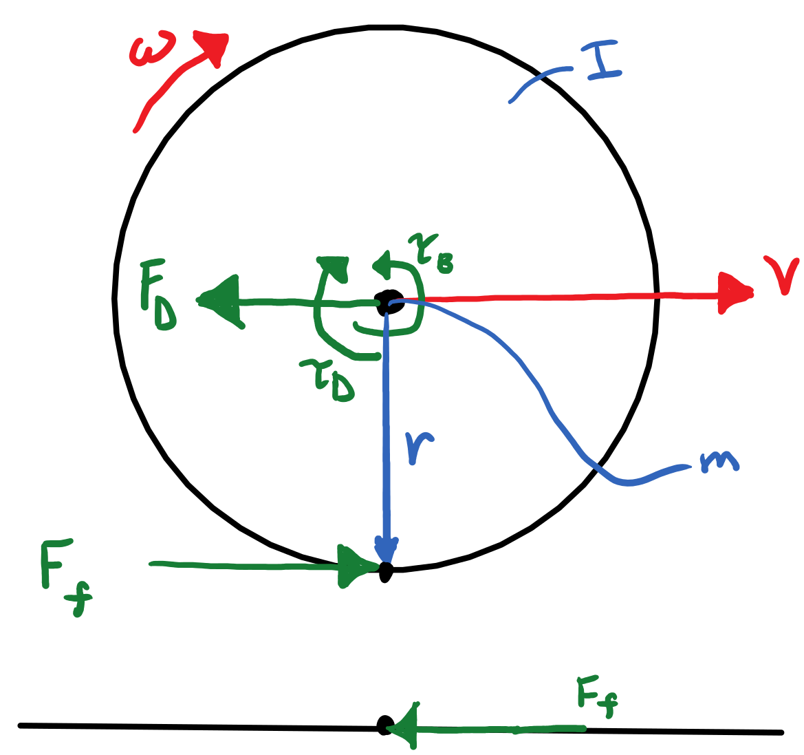
Figure 1: Schematics of the longitudinal car dynamics model.
The particle representing the car only has forward motion and its position is tracked by the time varying variable \(x\) as wells as its velocity \(v=\dot{x}\). The drag due to air resistance can be modeled by the drag equation:
The wheel can be modeled as a rotating disc with a radius equal to the effective rolling radius of the cars' tires \(r\). The rotational acceleration of the wheel is increased by an ideal applied torque \(\tau_D\) from the drivetrain. The rotational motion is resisted by bearing friction; modeled with a simple viscous damping model where \(b\) is the damping coefficient:
Lastly, there is a torque generated by the ground friction:
The friction force \(F_f\) can be modeled by a Coulomb-like equation which has a coefficient of friction \(\mu\) that varies with the drive slip ratio \(s_D\) and is proportional to the normal force \(F_N\) (the car's total weight in this case).
Equations of Motion
You will need to form Newton's Second Law and write it as two first order ODEs for the particle representing the car's longitudinal motion:
Next you will need to form Euler's Second Law for the wheel:
Make sure that you have correct signs on the elements of each summation above.
These can be written as four first order explicit ordinary differential equations:
These equations define expressions for the derivatives of the four time varying state variables \(x,v,\theta,\omega\) which are described below.
| Symbol | Description | Units |
|---|---|---|
| \(x\) | Longitudinal distance of the car | \(\textrm{m}\) |
| \(v\) | Longitudinal velocity of the car | \(\textrm{m/s}\) |
| \(\theta\) | Angle of the car's wheel | \(\textrm{rad}\) |
| \(\omega\) | Angular rate of the car's wheel | \(\textrm{rad/s}\) |
You will use the section Defining the State Derivative Function for these equations.
Inputs
The friction force \(F_f\) and the driving torque \(\tau_D\) should be treated as inputs to the above equations of motion. These input equations should be defined in a input function. See Time Varying Inputs for more information. The inputs function should take in the time, current state, and constants structure and produce a vector with \(\tau_D\), \(F_f\), \(s_D\), and \(\mu\).
Friction
The driving slip ratio \(s_D\) characterizes the actual forward velocity relative to the ideal pure rolling velocity and is defined as:
If \(v = \omega r\) there is no slip, i.e. pure rolling. If \(v < \omega r\) there is slip and the car does not advance as fast as it would if there were pure rolling. If \(s_D \geq 1\) the wheel is purely sliding on the ground (a burnout with no forward propulsion)
The longitudinal coefficient of friction \(\mu\) is a function of the slip ratio. This relationship is empirically derived for different tires and ground surface types. A mathematical model that does a good job at describing this relationship is:
where \(A,B,C,D\) are the coefficients that characterize the model's best fit to the empirical data. You are provided values for a typical tire on dry concrete and a typical tire on icy concrete in the "Constant Parameters" section below. Figure 2 shows the basic shape of these functions for dry concrete and icy concrete.
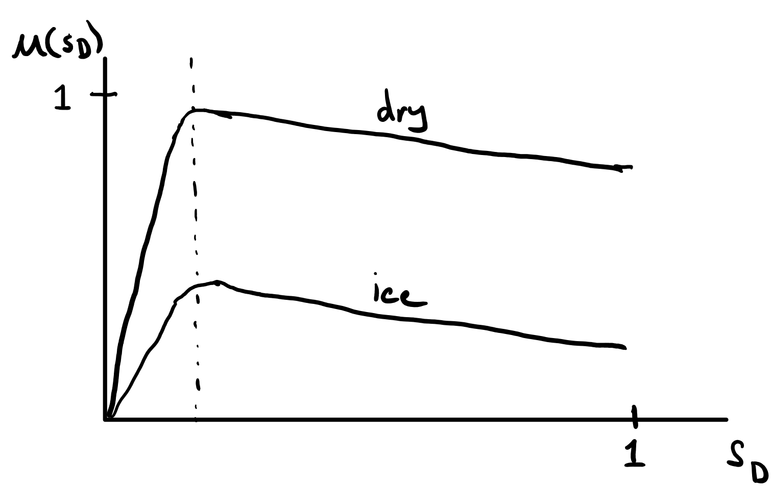
Figure 2: Typical relationship between the slip ratio and the coefficient of friction.
The race track will be 200 m long with a patch of ice between the 50 m and 100 m marks. You'll need to switch between the two sets of friction equation coefficients at the boundaries between dry and icy. You may be inclined to switch between these two conditions instantly, but numerical integration routines like ode45 are designed to work with continuous functions, so the switch between dry and ice and back will need to be a smooth transition. The logistic function provides a nice way to smoothly transition between two values. Below are the equations to calculate the coefficient values for any value of \(x\). You'll need to implement these using some form of control flow like an if-else or switch statement for each of the coefficients \(A,B,C,D\).
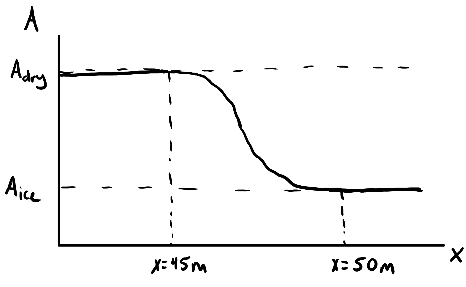
Figure 3: Use of the logistic function for a smooth transition between the coefficients.
The following shows the piecewise function for \(A\):
Driving torque
For the driving \(\tau_D\) you should consider two cases: without traction control and with traction control.
In the without traction control case, \(\tau_D\) should computed assuming the input power is a constant and always at its maximum \(P_{max}\). This assumes that the car's transmission is ideal and is always at the right gear ratio to operate at the engine's peak power output. \(\tau_D\) should then be governed by the current angular rate of the wheels \(\omega\). This models "flooring" the gas pedal and shifting the transmission perfectly to always maintain maximum power to the wheels.
For the traction control case, you will implement a simple proportional feedback traction control system that governs the torque by assuming you can measure the slip ratio and can calculate the error between it and a desired value \(s_{D peak} - s_D\). The driving torque will then be set to a gain \(k\) multiplied by the error. Thus torque will be increased with the error is growing and decreased when shrinking.
You'll need to determine the slip ratio that corresponds to the maximum coefficient of friction for the dry and icy conditions and use that for \(s_{D peak}\). Use the average of the dry and ice slip values as the \(s_{D peak}\) for simplicity. The gain \(k\) should be a positive value. You'll need to try different values to home in on the best performance for your car. Inspect the \(\mu\) and \(s_D\) curves versus time to see if this is behaving as expected. Also, the value of \(\tau_D\) produced by the controller should never cause the input power to be higher than \(P_{max}\). So always take the minimum of \(\tau_D\) in the without control case vs. the with control case to stay under the maximum power limit. In other words, the controller can't draw more power than \(P_{max}\).
Outputs
Your outputs should include all of the state trajectories and include the trajectories of the time varying slip ratio, coefficient of friction, driving torque, and friction force which have been computed already above in the state derivative and input functions. Additionally, compute the total energy consumed in traversing the 200 meter race distance. The time rate of change of the input energy is the input power which is related to the torque applied to the wheels and the angular rate of the wheels:
The input energy can be added as a fifth state variable to recover the total accumulated energy consumed. The trajectory of the power should also be added as an output variable.
You will use the section Outputs Other Than The States to compute these values. The outputs function should take in the time, current state, input function handle, and constants structure and produce a vector with \(\tau_D\), \(F_f\), \(s_D\), \(\mu\), \(P_{in}\).
Constant Parameters
The majority of the variables in the five differential equations and input equations above do not vary with time, i.e. they are constant. Below is a table with an explanation of each variable, its value, and its units. Note that the units are a self consistent set of SI base units.
| Symbol | Description | Value | Units |
|---|---|---|---|
| \(A_f\) | Car frontal area | \(0.5\) | \(\textrm{m}^2\) |
| \(C_D\) | Car drag coefficient | \(0.7\) | \(\textrm{unitless}\) |
| \(I\) | Combined spin moment of inerta of all four wheels | 2.0 | \(\textrm{kg}\cdot\textrm{m}^2\) |
| \(P_{max}\) | Maximum power available at the driveshaft | 745000 | \(\textrm{W}\) |
| \(b\) | Wheel viscous coefficient | 6.0 Note: This wass originally 30.0, but it was a error. | \(\textrm{N}\cdot\textrm{m}\cdot\textrm{s}\) |
| \(g\) | Acceleration due to gravity | 9.81 | \(\textrm{m/s}^2\) |
| \(k\) | Traction controller proportional gain | ? | \(\textrm{N}\cdot\textrm{m}\) |
| \(m\) | Mass of the car | 1000 | \(\textrm{kg}\) |
| \(r\) | Radius of the wheel | 0.2 | \(\textrm{m}\) |
| \(\rho\) | Density of air | 1.225 | \(\textrm{kg/m}^3\) |
| \(A_{dry}\) | Coefficient for friction equation | 0.9 | NA |
| \(B_{dry}\) | Coefficient for friction equation | 1.07 | NA |
| \(C_{dry}\) | Coefficient for friction equation | 28 | NA |
| \(D_{dry}\) | Coefficient for friction equation | 0.3 | NA |
| \(A_{ice}\) | Coefficient for friction equation | 0.1 | NA |
| \(B_{ice}\) | Coefficient for friction equation | 1.07 | NA |
| \(C_{ice}\) | Coefficient for friction equation | 38 | NA |
| \(D_{ice}\) | Coefficient for friction equation | 0.7 | NA |
You will use the section Integrating the Equations to for these values.
Initial Conditions
Start the car with an initial forward speed of 1 m/s (a rolling start) and set the wheel angular rate such that the wheel is purely rolling with no slip. All other states can be initialized as zero. See Integrating the Equations for how to set up the initial condition vector. Make sure that your initial conditions are arranged in the same order as your state variables.
Time Steps
Simulate the system for 10 seconds with time steps of 1/100th of a second. If your simulation is working with the provided constants you should see just over 300 meters of travel in 10 seconds.
Deliverables
In your lab report, show your work for creating and evaluating the simulation model. Include any calculations you had to do, for example those for state equations, initial conditions, input equations, time parameters, and any other parameters. Additionally, provide the indicated plots and answer the questions below. Append a copy of your Matlab/Octave code to the end of the report. The report should follow the report template and guidelines.
Submit a report as a single PDF file to Canvas by the due date that addresses the following items:
- Create a function defined in an m-file that evaluates the right hand side of the ODEs, i.e. evaluates the state derivatives. See Defining the State Derivative Function for an explanation.
- Create two functions defined each in an m-file that calculates the two requested inputs: with and without traction control. See Time Varying Inputs for an explanation.
- Create a function defined in an m-file that calculates the requested outputs. See Outputs Other Than the States for an explanation.
- Create a script in an m-file that utilizes the above functions to simulate system for the two scenarios: with and without traction control. This should setup the constants, integrate the dynamics equations, and plot each state, and output versus time. See Integrating the Equations for an explanation.
- Make a plot of the coefficients of friction versus slip ratio which includes the curves for the dry and icy conditions. Indicate what slip ratios were chosen for the peak traction.
- Make plots of the outputs versus time of the scenario without traction control and explain why you think the simulation is behaving realistically or unrealistically.
- Make plots to compare outputs versus time between the two scenarios: with and without traction control. Plotting the each trajectory on its own or in subplots with one color line for each scenario.
- Report the time to the 200 m mark for each scenario and discuss the results and explain why the vehicle that wins won. Report the input energy consumed at the 200 m mark and discuss the differences in energy consumption, why it is, and what the implications are. You can present the joules of energy in equivalent liters of gasoline to help get a idea of the quantity.
Tips
Make sure to construct the simulation in stages. Here is a good path:
- Create the state derivatives function.
- Create the inputs function with no traction control and no ice.
- Test the simulation till you are confident it is producing realistic results.
- Add ice to the input function. Test the simulation until it seems to be working.
- Create another input function with only control, no ice. Test the simulation until it seems to be working.
- Add both ice and control to the input function in 5. Test the simulation until it seems to be working.
- Create an outputs function and make your final plots.
Assessment Rubric
| Topic | [10 pts] Exceeds expectations | [5 pts] Meets expectatoins | [0 pts] Does not meet expectations |
|---|---|---|---|
| Functions | All Matlab/Octave functions are present and take correct inputs and produce the expected outputs. | Some of the functions are present and mostly take correct inputs and produce the expected outputs | No functions are present or not working at all. |
| Main Script | Constant parameters only defined once in main script(s); Integration produces the correct state, input, and output trajectories; Good choices in number of time steps and resolution are chosen and justified. | Parameters are defined in multiple places; Integration produces some correct state, input, and output trajectories; Poor choices in number of time steps and resolution are chosen | Constants defined redundantly; Integration produces incorrect trajectories; Poor choices in time duration and steps |
| Explanations | Explanation of two simulation comparisons are correct and well explained; Plots of appropriate variables are used in the explanations | Explanation of two simulation comparisons is somewhat correct and reasonably explained; Plots of appropriate variables are used in the explanations, but some are missing | Explanation of two simulations are incorrect and poorly explained; Plots are missing |
| Report and Code Formatting | All axes labeled with units, legible font sizes, informative captions; Functions are documented with docstrings which fully explain the inputs and outputs; Professional, very legible, quality writing; All report format requirements met | Some axes labeled with units, mostly legible font sizes, less-than-informative captions; Functions have docstrings but the inputs and outputs are not fully explained; Semi-professional, somewhat legible, writing needs improvement; Most report format requirements met | Axes do not have labels, legible font sizes, or informative captions; Functions do not have docstrings; Report is not professionally written and formatted; Report format requirements are not met |
| Contributions | Clear that all team members have made equitable contributions. | Not clear that contributions were equitable and you need to improve balance of contributions. | No indication of equitable contributions. |