Contents
Learning Objectives
After completing this lab you will be able to:
- formulate the explicit first order ordinary differential equations for the roll and steer dynamics of a bicycle
- translate ordinary differential equations into a computer function that evaluates the equations at any given point in time
- develop a function that evaluates state dependent input functions
- develop a function that evaluates state and input dependent output variables
- numerically integrate ordinary differential equations with Octave/Matlab's ode45
- create complete and legible plots of the resulting input, state, and output trajectories
- create a report with textual explanations and plots of the simulation
- evaluate a bicycle model for stability at different speeds
- design a feedback controller that stabilizes a bicycle at different speeds
- design a bicycle that is self-stable at low speeds
Information
Extra information (asides) are in blue boxes.
Warnings
Warnings are in yellow boxes.
Introduction
In this lab, you will investigate the dynamics of a bicycle with and without a controller to assist in balancing. Bicycles and motorcycles share the same core dynamic behavior, so this lab will introduce you to phenomena that apply to both vehicles. Below is a video that demonstrates a bicycle's uncanny ability to be self-stable, i.e. return to an upright configuration even when perturbed from its equilibrium. This is, of course, not always possible as we know that a bicycle will simply fall over if it has no forward speed and we also know that bicycles require some control from the rider in general. In this lab, you will simulate the Whipple-Carvallo bicycle model, investigate its dynamics, apply a controller to stabilize it at low speeds, and design a bicycle that can self-stabilize at lower speeds.
System Description
The Whipple-Carvallo bicycle model is essentially the simplest model that behaves like a bicycle and can exhibit self-stability. "Self-stability" is defined as open loop stability or stability without any control inputs. The model was developed by both Whipple and Carvallo around the turn of the 20th century. In 2007, Meijaard, Papdopoulos, Ruina, and Schwab validated the model and presented a benchmark formulation [Meijaard2007]. You'll be using this formulation for the lab. This model assumes no-slip non-deforming tires, a flat level surface, frictionless revolute joints, and a human rider that is rigidly fixed to the rear bicycle frame. See the cited paper for more details about the history of the model, its derivation, and in-depth analysis. Figure 1 shows the basic geometry and the four rigid bodies: [B] rear frame and human body, [H] handlebar and fork, [R] rear wheel, and [F] front wheel.
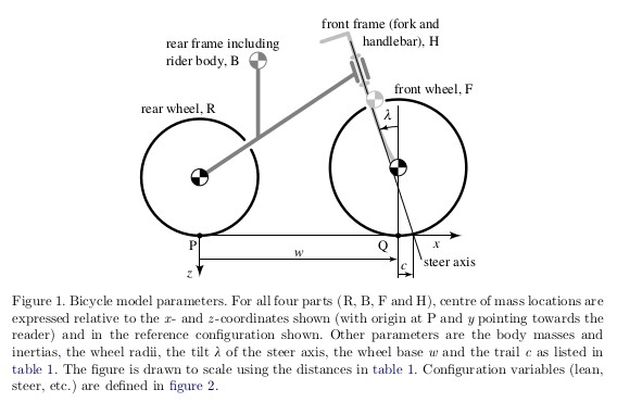
Figure 1: Schematic of the benchmark bicycle model.
| [Meijaard2007] | J.P Meijaard, Jim M Papadopoulos, Andy Ruina and A.L Schwab, 2007, Linearized dynamics equations for the balance and steer of a bicycle: a benchmark and review, Proc. R. Soc. A. 4631955–1982 http://doi.org/10.1098/rspa.2007.1857 |
Equations of Motion
The equations of motion for the Whipple-Carvallo benchmark bicycle model are presented below in a canonical-like linear form:
where
The time varying variables are:
| Symbol | Description | Units |
|---|---|---|
| \(\phi\) | Roll angle of the bicycle's rear frame relative to the ground. Positive about the x axis (rightward lean). | \(\textrm{rad}\) |
| \(\delta\) | Steer angle; angle between handlebar + fork and rear frame. Positive is rotation about the ~z axis (rightward steer). | \(\textrm{rad}\) |
| \(\omega=\dot{\phi}\) | Roll angular rate. | \(\textrm{rad/s}\) |
| \(\beta=\dot{\delta}\) | Steer angular rate. | \(\textrm{rad/s}\) |
| \(T_\phi\) | Roll torque (between ground and rear frame) | \(\textrm{N}\cdot\textrm{m}\) |
| \(T_\delta\) | Steer torque (between rear frame and handlebar + fork) | \(\textrm{N}\cdot\textrm{m}\) |
You will need to formulate the equations of motion as four explicit linear ordinary differential equations in first order form for your state derivative function. The state space form is a good best way to do this:
where
Use matrix algebra to determine \(A\) and \(B\) from the canonical form matrices.
You will use the section Defining the State Derivative Function for these equations.
Inputs
You will examine two inputs scenarios:
- No control
- \(T_\phi\) and \(T_\delta\) should both be set to zero for all time. These inputs will be used to examine the self-stability of the bicycle.
- Roll rate feedback control
Define an input function that applies a steer torque \(T_\delta\) proportional to the negative roll angular rate. This is a classic "negative feedback" controller that will attempt to drive the roll rate to zero. The controller equation is:
\begin{equation*} T_\delta = -k\omega \end{equation*}
See Time Varying Inputs for more information.
Outputs
The output function should return all of the state variables and the steering torque input. Include these five time varying variables in your simulation plots. You will use the section Outputs Other Than The States to compute these values.
Constant Parameters
The majority of the variables in the differential equations and input equations above do not vary with time, i.e. they are constant. Below is a table with an explanation of each variable, its value, and its units. Note that the units are a self consistent set of SI base units. The values given represent a typical bicycle and rider.
| Symbol | Matlab variable | Description | Value | Units |
|---|---|---|---|---|
| \(I_{Bxx}\) | IBxx | Rear frame and human body x moment of inertia | 9.2 | \(\textrm{kg}\cdot\textrm{m}^2\) |
| \(I_{Bxz}\) | IBxz | Rear frame and human body xz product of inertia | 2.4 | \(\textrm{kg}\cdot\textrm{m}^2\) |
| \(I_{Byy}\) | IByy | Rear frame and human body y moment of inertia | 11.0 | \(\textrm{kg}\cdot\textrm{m}^2\) |
| \(I_{Bzz}\) | IBzz | Rear frame and human body z moment of inertia | 2.8 | \(\textrm{kg}\cdot\textrm{m}^2\) |
| \(I_{Fxx}\) | IFxx | Front wheel radial moment of inertia | 0.1405 | \(\textrm{kg}\cdot\textrm{m}^2\) |
| \(I_{Fyy}\) | IFyy | Front wheel spin moment of inertia | 0.28 | \(\textrm{kg}\cdot\textrm{m}^2\) |
| \(I_{Hxx}\) | IHxx | Handlebar and fork x moment of inertia | 0.05892 | \(\textrm{kg}\cdot\textrm{m}^2\) |
| \(I_{Hxz}\) | IHxz | Handlebar and fork xz product of inertia | -0.00756 | \(\textrm{kg}\cdot\textrm{m}^2\) |
| \(I_{Hyy}\) | IHyy | Handlebar and fork y moment of inertia | 0.06 | \(\textrm{kg}\cdot\textrm{m}^2\) |
| \(I_{Hzz}\) | IHzz | Handlebar and fork z moment of inertia | 0.00708 | \(\textrm{kg}\cdot\textrm{m}^2\) |
| \(I_{Rxx}\) | IRxx | Rear wheel radial moment of inertia | 0.0603 | \(\textrm{kg}\cdot\textrm{m}^2\) |
| \(I_{Ryy}\) | IRyy | Rear wheel spin moment of inertia | 0.12 | \(\textrm{kg}\cdot\textrm{m}^2\) |
| \(c\) | c | Trail | 0.08 | \(\textrm{m}\) |
| \(g\) | g | Acceleration due to gravity | 9.81 | \(\textrm{m/s}^2\) |
| \(\lambda\) | lambda | Steer axis tilt | \(\pi/10\) | \(\textrm{rad}\) |
| \(m_B\) | mB | Mass of rear frame and human body | 85.0 | \(\textrm{kg}\) |
| \(m_F\) | mF | Mass of front wheel | 3.0 | \(\textrm{kg}\) |
| \(m_H\) | mH | Mass of handlebar and fork | 4.0 | \(\textrm{kg}\) |
| \(m_R\) | mR | Mass of rear wheel | 2.0 | \(\textrm{kg}\) |
| \(r_F\) | rF | Radius of front wheel | 0.35 | \(\textrm{m}\) |
| \(r_R\) | rR | Radius of rear wheel | 0.3 | \(\textrm{m}\) |
| \(w\) | w | Wheelbase | 1.02 | \(\textrm{m}\) |
| \(x_B\) | xB | Rear frame and human body mass center x coordinate | 0.3 | \(\textrm{m}\) |
| \(x_H\) | xH | Handlebar and fork mass center x coordinate | 0.9 | \(\textrm{m}\) |
| \(z_B\) | zB | Rear frame and human body mass center z coordinate | -0.9 | \(\textrm{m}\) |
| \(z_H\) | zH | Handlebar and fork mass center z coordinate | -0.7 | \(\textrm{m}\) |
| \(v\) | v | Speed, positive is forward. | varies | \(\textrm{m/s}\) |
| \(k\) | k | Control gain | varies | \(\textrm{Nms}\) |
The following function compute_benchmark_bicycle_matrices.m computes \(\mathbf{M,C1,K0,K2}\) given a structure with the above constant parameters defined. Use this function along with your m-files to setup your model.
function [M, C1, K0, K2] = compute_benchmark_bicycle_matrices(p)
% COMPUTE_BENCHMARK_BICYCLE_MATRICES - Returns the canonical matrices of the
% benchmark Whipple-Carvallo bicycle model linearized about the upright
% constant velocity configuration. It uses the parameter definitions from:
%
% J.P Meijaard, Jim M Papadopoulos, Andy Ruina and A.L Schwab, 2007,
% Linearized dynamics equations for the balance and steer of a bicycle: a
% benchmark and review, Proc. R. Soc. A. 4631955–1982
% http://doi.org/10.1098/rspa.2007.1857
%
% Syntax: [M, C1, K0, K2] = compute_benchmark_bicycle_matrices(p)
%
% Inputs:
% p - structure
%     A dictionary of the benchmark bicycle parameters. Make sure your units
%     are correct and match the benchmark paper's units.
%
% Outputs:
% M - matrix, size 2x2
%     The mass matrix.
% C1 - matrix, size 2x2
%     The part of the damping matrix that is proportional to the speed, v.
% K0 - matrix, size 2x2
%     The part of the stiffness matrix proportional to gravity, g.
% K2 - matrix, size 2x2
%     The part of the stiffness matrix proportional to the speed squared,
%     v^2.

mT = p.mR + p.mB + p.mH + p.mF;
xT = (p.xB*p.mB + p.xH*p.mH + p.w*p.mF)/mT;
zT = (-p.rR*p.mR + p.zB*p.mB + p.zH*p.mH - p.rF*p.mF)/mT;

ITxx = (p.IRxx + p.IBxx + p.IHxx + p.IFxx + p.mR*p.rR^2 + p.mB*p.zB^2 + ...
        p.mH*p.zH^2 + p.mF*p.rF^2);
ITxz = (p.IBxz + p.IHxz - p.mB*p.xB*p.zB - p.mH*p.xH*p.zH + p.mF*p.w*p.rF);
p.IRzz = p.IRxx;
p.IFzz = p.IFxx;
ITzz = (p.IRzz + p.IBzz + p.IHzz + p.IFzz + p.mB*p.xB^2 + p.mH*p.xH^2 + ...
        p.mF*p.w^2);

mA = p.mH + p.mF;
xA = (p.xH*p.mH + p.w*p.mF)/mA;
zA = (p.zH*p.mH - p.rF*p.mF)/mA;

IAxx = (p.IHxx + p.IFxx + p.mH*(p.zH - zA)^2 + p.mF*(p.rF + zA)^2);
IAxz = (p.IHxz - p.mH*(p.xH - xA)*(p.zH - zA) + p.mF*(p.w - xA)*(p.rF + ...
        zA));
IAzz = (p.IHzz + p.IFzz + p.mH*(p.xH - xA)^2 + p.mF*(p.w - xA)^2);
uA = (xA - p.w - p.c)*cos(p.lambda) - zA*sin(p.lambda);
IAll = (mA*uA^2 + IAxx*sin(p.lambda)^2 + 2*IAxz*sin(p.lambda)*cos(p.lambda) + ...
        IAzz*cos(p.lambda)^2);
IAlx = (-mA*uA*zA + IAxx*sin(p.lambda) + IAxz*cos(p.lambda));
IAlz = (mA*uA*xA + IAxz*sin(p.lambda) + IAzz*cos(p.lambda));

mu = p.c/p.w*cos(p.lambda);

SR = p.IRyy/p.rR;
SF = p.IFyy/p.rF;
ST = SR + SF;
SA = mA*uA + mu*mT*xT;

Mpp = ITxx;
Mpd = IAlx + mu * ITxz;
Mdp = Mpd;
Mdd = IAll + 2*mu*IAlz + mu^2*ITzz;
M = [Mpp, Mpd; Mdp, Mdd];

K0pp = mT*zT;
K0pd = -SA;
K0dp = K0pd;
K0dd = -SA*sin(p.lambda);
K0 = [K0pp, K0pd; K0dp, K0dd];

K2pp = 0.0;
K2pd = (ST - mT*zT)/p.w*cos(p.lambda);
K2dp = 0.0;
K2dd = (SA + SF*sin(p.lambda))/p.w*cos(p.lambda);
K2 = [K2pp, K2pd; K2dp, K2dd];

C1pp = 0.0;
C1pd = (mu*ST + SF*cos(p.lambda) + ITxz/p.w*cos(p.lambda) - mu*mT*zT);
C1dp = -(mu*ST + SF*cos(p.lambda));
C1dd = (IAlz/p.w*cos(p.lambda) + mu*(SA + ITzz / p.w*cos(p.lambda)));
C1 = [C1pp, C1pd; C1dp, C1dd];

end
You will use the section Integrating the Equations to for these values.
Initial Conditions
For the simulations, set the initial conditions as:
This will start the vehicle off with a small roll and steer angle. See Integrating the Equations for how to set up the initial condition vector. Make sure that your initial conditions are arranged in the same order as your state variables.
Time Steps
Simulate the system for 5 seconds with time steps of 1/100th of a second.
Eigenvalues and Stability
Matlab and Octave can easily calculate the roots of the characteristic equation, i.e. the eigenvalues, given a state dynamics matrix \(\mathbf{A}\). The eig() function calculates the eigenvalues. It is used like so:
evals = eig(A);
The variable evals will then contain a vector of eigenvalues. The functions real() and imag() are also helpful to extract the real and imaginary parts of the complex eigenvalues.
See the Matlab documentation for more about these functions:
- https://www.mathworks.com/help/matlab/ref/eig.html
- https://www.mathworks.com/help/matlab/ref/real.html
- https://www.mathworks.com/help/matlab/ref/imag.html
Plotting the eigenvalues
The bicycle's stability is speed dependent, so it will be useful to plot the real part of the eigenvalues versus the speed \(v\) to determine this relationship. Make sure to only plot a dot for each data point, otherwise you'll get a very hard to interpret plot, e.g.:
plot(speeds, real_part_of_evals, '.')
Using a Root Locus To Choose a Feedback Gain
A root locus is a parametric plot of the complex plane that shows how the roots of the characteristic equation change with respect to changes in a single parameter in a linear model. Any parameter can be chosen but the most common parameter is a proportional control gain of a closed loop negative feedback controller. It turns out that the Whipple-Carvallo bicycle model can be stabilized by "steering into the fall". One way to formalize this statement is to apply steer torque in the direction of the roll angular rate, i.e. if you roll towards the right, steer towards the right. You'll first need to determine the transfer function that relates the steer torque input \(T_\delta\) to the roll angular rate \(\omega\):
You can use Cramer's rule to find this transfer function, as in the book, or there are various Matlab/Octave functions that can help, for example ss2tf() can convert a state space system to equivalent transfer functions. If you use Cramer's rule you'll need to use the tf() function to construct the transfer function in Matlab/Octave. There isn't any reason to do any algebra by hand, use Matlab/Octave to do the number crunching.
Once you have a transfer function you can use the rlocus() function to make a standard root locus plot as a function of the negative feedback gain \(k\). You'll need to examine this plot to determine what gain value ensures that all roots are in the left half of the complex plane.
- https://www.mathworks.com/help/matlab/ref/ss2tf.html
- https://www.mathworks.com/help/matlab/ref/tf.html
- https://www.mathworks.com/help/control/ref/tf.rlocus.html
Sign of the feedback gain
The root locus function assumes a negative feedback gain, i.e. that \(T_\delta=-k\omega\), thus you provide a positive value of the gain to get negative feedback. Think very carefully about the "steer into the fall" and the sign conventions of the state variables. You'll need to setup your root locus to examine gains that cause a "steer into the fall".
Checking your work
You can use the BicycleParameters web app to visualize the bicycle geometry and to double check your eigenvalue plots. Visit the app here:
http://bicycleparameters.herokuapp.com/
This app was recently developed by a UCD physics undergraduate, Noah Sanders, and is powered by similar calculations that you are doing in this lab. It is still in beta and there may be some bugs, but you should be able to edit the parameters in the table to see changes in the two figures.
Deliverables
In your lab report, show your work for creating and evaluating the simulation model. Include any calculations you had to do, for example those for state equations, initial conditions, input equations, time parameters, and any other parameters. Additionally, provide the indicated plots and answer the questions below. Append a copy of your Matlab/Octave code to the end of the report. The report should follow the report template and guidelines.
Submit a report as a single PDF file to Canvas by the due date that addresses the following items:
Create a function defined in an m-file that evaluates the right hand side of the ODEs, i.e. evaluates the state derivatives. See Defining the State Derivative Function for an explanation.
Create two functions defined each in an m-file that calculates the two requested inputs: no control and with control. See Time Varying Inputs for an explanation.
Create a function defined in an m-file that calculates the requested outputs. See Outputs Other Than the States and Outputs Involving State Derivatives for an explanation.
Create a script in an m-file that utilizes the above functions to simulate system for the scenarios described below. This should setup the constants, integrate the dynamics equations, and plot each state, and output versus time. See Integrating the Equations for an explanation.
Make a plot where the Y axis is the real part of the eigenvalues (determines growth or decay and the rate) and the X axis is the bicycle speed. The speeds should vary from 0 to 10 m/s (0 to ~22 mph). Discuss how the bicycle's self-stability relates to the speed and discuss any speed values that stand out and what the eigenvalues at this speed tell you about the motion. Use simulation (states vs time: 0 to 5 seconds) plots to back up your explanations at the particular speeds of interest. Be sure to explain your simulation plots in terms of growth/decay rates, oscillation frequencies, and phase differences in the states. Limit your Y axis to +/- 90 degs for unstable simulations.
Develop two roll feedback controllers using a root locus to select an appropriate gain to stabilize the bicycle at 2 m/s and 8 m/s. At 2 m/s feedback roll rate. At 8 m/s feedback roll angle. Both controllers should control steer torque. Choose gains that give realistic decay rates and oscillation frequencies (a human's arm control bandwidth has an upper bound of about 10 rad/s). Simulate the system at these speeds with the controller defined in an input function to show that the system is stable. Discuss the sign of the gain values.
Design a bicycle by changing any number of the parameters values so that it is self-stable (no control) at a very low range of speeds. Try not to choose parameter values that would be impossible to actually build, e.g. a wheelbase that is 100 meters long or rear frame/human mass of 1 kg. There is no single solution to this. Once you chose a bike, simulate it at a very low speed and discuss the simulation results and the advantages/disadvantages of the bicycle design. A practical use of a bicycle that is self-stable at low speeds could be to make it easy for people to learn to ride a bicycle. The videos below show bicycles designed for low-speed stability:
Assessment Rubric
| Topic | [10 pts] Exceeds expectations | [5 pts] Meets expectatoins | [0 pts] Does not meet expectations |
|---|---|---|---|
| Functions | All Matlab/Octave functions are present and take correct inputs and produce the expected outputs. | Some of the functions are present and mostly take correct inputs and produce the expected outputs | No functions are present or not working at all. |
| Main Script | Constant parameters only defined once in main script(s); Integration produces the correct state, input, and output trajectories; Good choices in number of time steps and resolution are chosen and justified; Intermediate calculations present and functioning. | Parameters are defined in multiple places; Integration produces some correct state, input, and output trajectories; Poor choices in number of time steps and resolution are chosen; Intermediate calculations mostly present and functioning. | Constants defined redundantly; Integration produces incorrect trajectories; Poor choices in time duration and steps; Intermediate calculations not present or functioning. |
| Eigenvalue plot | Eigenvalue vs. speed plot is correct; At least three unique speeds identified and the behavior at each speed is explained via simulation plots and a correct explanation. | Eigenvalue vs. speed plot is mostly correct; As least one unique speed is identified and the behavior at that speed is explained via simjulation plots and reasonably explanation. | No eigenvalue vs. speed plot present and no simulations created for unique speeds. No explanations. |
| Control | Roll rate feedback controller functions and a root locus plot is shown and used to select an appropriate gain. Simulations show stability at each speed and comments on the gain values at each speed are provided. | Roll rate feedback controller functions but no root locus plot is shown and used to select an appropriate gain. Simulations mostly show stability at each speed or some speeds are missing; Comments on the gain values at most speeds are provided. | Roll rate feedback controller does not function; Not apparent that a root locus was used to select an appropriate gain; No comments on the gains at each speed. |
| Bicycle design | A realistic bicycle design is selected that is self-stable at lower speeds and the parameter selection is explained and justified. Stability is proven by the eigevalues or simulations. Valid explanation of the design's advantages and disadvantages is present. | A non-realistic bicycle design is selected that is self-stable at lower speeds and the parameter selection may not be explained and justified. Stability is proven by the eigevalues or simulations. Explationan of the design's advantages and disadvantages is present. | No bicycle is shown that is self-stable at lower speeds. No explanation of the designs are present. |
| Report and Code Formatting | All axes labeled with units, legible font sizes, informative captions; Functions are documented with docstrings which fully explain the inputs and outputs; Professional, very legible, quality writing; All report format requirements met | Some axes labeled with units, mostly legible font sizes, less-than-informative captions; Functions have docstrings but the inputs and outputs are not fully explained; Semi-professional, somewhat legible, writing needs improvement; Most report format requirements met | Axes do not have labels, legible font sizes, or informative captions; Functions do not have docstrings; Report is not professionally written and formatted; Report format requirements are not met |
| Contributions | Clear that all team members have made equitable contributions. | Not clear that contributions were equitable and you need to improve balance of contributions. | No indication of equitable contributions. |