Contents
Learning Objectives
After completing this lab you will be able to:
- derive the equations of motion for longitudinal drone flight dynamics
- formulate the explicit first order ordinary differential equations for the system
- translate ordinary differential equations into a computer function that evaluates the equations at any given point in time
- develop a function that evaluates state dependent input functions
- develop a function that evaluates state and input dependent output variables
- numerically integrate ordinary differential equations with Octave/Matlab's ode45
- create complete and legible plots of the resulting input, state, and output trajectories
- create a report with textual explanations and plots of the simulation
- design a PID controller that stabilizes the drone in pitch and tracks a path
Information
Extra information (asides) are in blue boxes.
Warnings
Warnings are in yellow boxes.
Introduction
In this lab, you will investigate the longitudinal (altitude and pitch) flight dynamics of a quadcopter traveling at a constant forward speed. This vehicle relies completely on the independently controlled thrust generated by pairs of rotors at the front and rear of the vehicle to change altitude and its pitch orientation. The vehicle is very much unstable and requires controllers to maintain a desired pitch angle and to control altitude. The following video shows an autonomous quadcopter that can avoid obstacles using a combination of vision detection to determine relative locations of the obstacles and a feedback controller to avoid the obstacles given the computed desired path of motion. You will develop the feedback controller portion of a system like the one shown.
Here is another similar system using a fixed wing autonomous aircraft at higher speeds:
System Description
You will model the longitudinal dynamics of a drone flying at a constant forward speed \(U\). The vehicle can be modeled as a single rigid body with pitch centroidal moment of inertia \(I\) and mass \(m\). Use an inertial coordinate system with coordinate \(x\) to measure the horizontal travel and coordinate \(z\) for the vertical travel. Use the standard of positive \(z\) pointing downwards. The front rotors are separated from the rear rotors by distance \(a + b\) and the mass center lies at distance \(a\) from the front rotor and distance \(b\) from the rear rotor.
The mass center will have a velocity \(U\) in the \(x\) direction which is constant and a variable velocity \(W\) in the vertical direction. The rigid body will have a pitch angle \(\theta\) and a pitch angular velocity \(q\).
The vehicle will have four forces acting on it. The two pairs of rotors produce the thrust force \(F_f\) at the front of the vehicle and the rotors at the rear produce thrust force \(F_r\). The weight of the vehicle \(mg\) is the third force and the fourth force is the drag force acting perpendicular to the quadcopter's body \(F_D\) at the center of pressure (equal to aerodynamic center in this case) which is equidistant from the to rotors. The drag force should be modeled by the equation:
This drag force will not affect motion in the \(x\) direction since \(U\) is specified to be constant but you will need to determine its contribution to resisting vertical motion. Make sure that the force is always in the opposite direction of the component of \(\bar{v} = U \hat{x} + W \hat{z}\) that is perpendicular to the vehicle (same as \(F_D\)) using the signum function, sign() in Matlab/Octave. Neglect any lift that may be produced due to the vehicles angle of attack or body characteristics.
What is \(v\) in the drag equation?
\(v\) in the equation for \(F_D\) is the scalar component of velocity of the center of pressure (CoP) that is parallel to \(F_D\). If you write the velocity vector of the CoP in the body fixed reference frame you can get this component like we have for other body fixed velocity calculations.
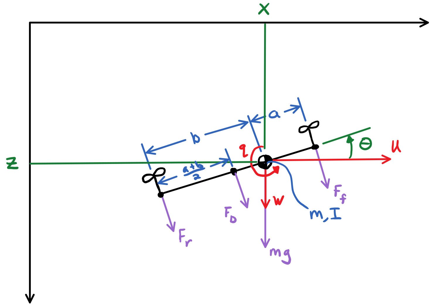
Figure 1: Schematics of the longitudinal quadcopter dynamics. The vectors are all drawn with a common sign convention, positive in the direction of the arrow.
Equations of Motion
You will need to derive the equations of motion for this system. Using the coordinates described above write the non-linear Newton-Euler equations. You will be expected to show this work in your report. Note: Use inertial coordinates not body fixed for the derivation. There will be two equations, one for vertical deviation from equilibrium and one for pitch deviation from equilibrium.
\(x\) acceleration equation
There is no acceleration in the \(x\) direction so you do not write an equation for that coordinate. This is because we are imposing the assumption that the thrust is always the perfect amount to maintain constant forward speed irrespective of the pitch angle and thrust contributions from the rotors.
It will be useful to rewrite the two force magnitudes in terms of the total force \(F_T = F_f + F_r\) so that you can control \(F_T\) to control altitude and regulate \(F_f\) for pitch control. Eliminate \(F_r\) from the two equations.
The state and input vectors would then be:
The time varying variables are:
| Symbol | Description | Units |
|---|---|---|
| \(z\) | Vertical coordinate of the quadcopter's mass center | \(\textrm{m}\) |
| \(\theta\) | Pitch angle. | \(\textrm{rad}\) |
| \(w=\dot{z}\) | Vertical velocity | \(\textrm{m/s}\) |
| \(q=\dot{\theta}\) | Pitch angular rate | \(\textrm{rad/s}\) |
| \(F_T\) | Total thrust produced by the rotors | \(\textrm{N}\) |
| \(F_f\) | Thrust produced by the front rotors | \(\textrm{N}\) |
You will need to formulate the equations of motion as four explicit linear ordinary differential equations in first order form for your state derivative function.
You will use the section Defining the State Derivative Function for these equations.
Inputs
The quadcopter will simply spin to its death as it falls to the ground without any control. You will develop two Proportional-Integral-Derivative (PID) controllers. One will be used to stabilize the vehicle in the pitch degree of freedom and maintain level flight. The second will be used to maintain a desired altitude. Your input function should return the two forces \(F_T\) and \(F_f\). The controllers take this form in the time domain:
Derivative term
You may wonder why \(q\) and \(w\) are in the above equations. Note that:
The PID controllers have three terms:
- Proportional term
- Applies control that is proportional to the error: desired minus the actual. This term gives a spring-like effect to your controller, e.g. the larger the pitch angle is away from the desired the more force the controller applies to force the pitch angle to the desired angle \(\theta_d\).
- Integral term
- Applies control that is proportional the integral of the error. This term is included to reduce or eliminate steady state error in the step response of the controlled system.
- Derivative term
- Applies control that is proportional to the derivative of the error. This term provides a damping effect to the controlled variable which can control overshoot and even eliminate oscillation for a critically damped response. The desired rates should all be zero only desired coordinates need be set.
There are techniques to select PID gains for a known linear plant model that have a desired step response. You have or will learn about these in EME 172. You can also design a controller with manually tuning for a non-linear system that has reasonable number of inputs and outputs, which we have with this drone model. Watch the video below to get an idea of how one can systemically tune a PID controller for desired performance by first trying P gains to get a stable response, then D gains to reduce oscillations, and I gains to reduce steady state error.
Once you have your systems simulating with no control (the drone should fall to the ground spinning chaotically), follow these steps:
- Set \(F_T\) to a constant value. If you choose a value close to the weight of the vehicle the drone should have enough total force to try to approximately hover.
- Set the desired pitch angle to a constant value \(\theta_d = \pi/180\) so that you will get a step response for \(\theta\).
- Apply the technique in the video to the control equation for \(F_f\). This should allow you to stabilize the quadcopter in pitch with a good response and it will either slowly fall or rise depending on the value you set \(F_T\) to. Remember the sign convention of \(F_f\) and that this is negative feedback to ensure you choose the right sign of the gains. The simulation only needs about 5 seconds of simulation time for the tuning process.
- Set the \(F_f\) gains to the ones you found in 3 and set the desired altitude to a constant value \(z_d = -1\) so that you you will get a step response for \(z\). Set \(\theta_d = 0\) for level flight.
- Apply the technique in the video to the control equation for \(F_T\) until you get a good step response for altitude \(z\).
Integral of the error
The proportional and derivative error terms are straight forward but how do you obtain the integral of the error?
Recall that ode45 integrates equations with respect to time. You need to integrate the error with respect to time from \(t=0\) to the current time \(t\) to obtain the cumulative error in the controller. To do so you can introduce two new state variables for the cumluative error \(\theta_c\) and \(z_c\). Add these two state equations to your state derivative right hand side function like so:
Note that the computed states are then the term you desire:
If you can't get this part working you can still control the vehicle with two PD controllers, you'll just have stead state error.
Once you have selected all six gains and have good simultaneous step responses for \(\theta\) and \(z\) you can now track an altitude "path" for a 20 second simulation. Setup your input function to have a desired altitude of:
Simulate the controlled system for this input and plot all the requested output variables.
Plotting with z positive downward
For the plots that include \(z\) and \(w\) on the plot's ordinate axis it is helpful to reverse the axis so the negative values are above the positive values. To do so you can use this code after you call plot():
h = gca;  % gets a handle to the most recent axis
set(h, 'YDir', 'reverse');  % reverses the ordinate
See Time Varying Inputs for more information.
Constant Parameters
The majority of the variables in the differential equations and input equations above do not vary with time, i.e. they are constant. Below is a table with an explanation of each variable, its value, and its units. Note that the units are a self consistent set of SI base units.
| Symbol | Matlab variable | Description | Value | Units |
|---|---|---|---|---|
| \(I\) | I | Centroidal pitch moment of inertia | Calculate and use the moment of inertia of a slender rod of mass \(m\) and length \(a + b\) with a mass center equidistant from the ends. You can find this in a moment of inerta table. | \(\textrm{kg}\cdot\textrm{m}^2\) |
| \(a\) | a | Distance from front rotor to mass center | 0.1 | \(\textrm{m}\) |
| \(b\) | b | Distance from rear rotor to mass center | 0.2 | \(\textrm{m}\) |
| \(g\) | g | Acceleration due to gravity | 9.81 | \(\textrm{m/s}^2\) |
| \(m\) | m | Mass of the quadcopter | 1.0 | \(\textrm{kg}\) |
| \(U\) | U | Forward speed of the quadcopter | 15 | \(\textrm{m/s}\) |
| \(\rho\) | rho | Density of air | 1.225 | \(\textrm{kg}/m^s\) |
| \(A\) | A | Top view area of the quadcopter | Assume a square shape | \(\textrm{m}^2\) |
| \(C_D\) | CD | Drag coefficient | 0.1 | Unitless |
| \(k_{fp}\) | kfp | Front rotor force proportional control gain | Determined by you | \(\textrm{N/rad}\) |
| \(k_{fi}\) | kfi | Front rotor force integral control gain | Determined by you | \(\textrm{N/rad/s}\) |
| \(k_{fd}\) | kfd | Front rotor force derivative control gain | Determined by you | \(\textrm{Ns/rad}\) |
| \(k_{Tp}\) | kTp | Total rotor force proportional control gain | Determined by you | \(\textrm{N/rad}\) |
| \(k_{Ti}\) | kTi | Total rotor force integral control gain | Determined by you | \(\textrm{N/rad/s}\) |
| \(k_{Td}\) | kTd | Total rotor force derivative control gain | Determined by you | \(\textrm{Ns/rad}\) |
You will use the section Integrating the Equations to for these values.
Outputs
The output function should return all six of the state variables, the travel distance \(x\), the two rotor forces \(F_f,F_r\), and the desired altitude \(z_d\). Include these ten time varying variables in your simulation plots. You will use the section Outputs Other Than The States to compute these values.
Initial Conditions
For the simulations, set the initial conditions all to zero.
See Integrating the Equations for how to set up the initial condition vector. Make sure that your initial conditions are arranged in the same order as your state variables.
Time Steps
Simulate the system for 20 seconds with time steps of 1/20th of a second for all simulations.
Animation
The following function animate_drone.m function will create an animation of your drone flight simulation. You can use this to visualize the simulation and assess the controller's performance.
function animate_drone(ts, ys, p)
% ANIMATE_DRONE - Creates an animation of the drone flight given the output
% trajectories.
%
% Syntax: animate_drone(ts, ys, p)
%
% Inputs:
%   ts - Vector of time values, size 1x1000.
%   ys - Matrix of output values , size 1000x10
%        The outputs are, in order:
%        1: theta, pitch angle [rad]
%        2: z, altitude [m]
%        3: q, pitch rate [rad/s]
%        4: w, vertical velocity [m/s]
%        5: thetac, cumlative pitch error [rad]
%        6: zc, cumlative altitude error [rad]
%        7: Ff, Front rotor thrust [N]
%        8: Fr, Rear rotor thrust [N]
%        9: x, longitudinal position [m]
%        10: zd, desired altitude [m]
%   p - Constant parameter structure that includes at least a and b.

figure()
hold on
box on

extents = 2.0;  % meters

delt = ts(2) - ts(1);

thetas = ys(:, 1);
zs = ys(:, 2);
xs = ys(:, 9);
zds = ys(:, 10);

desired_path = plot(xs(1:2), zds(1:2), 'r');
actual_path = plot(xs(1:2), zs(1:2), 'b');

for i = 2:length(ts)
    theta = thetas(i);
    z = zs(i);
    x = xs(i);
    % update the desired path
    set(desired_path, 'XData', xs(1:i), 'YData', zds(1:i));
    % update the acutal path
    set(actual_path, 'XData', xs(1:i), 'YData', zs(1:i));
    % plot the "wings"
    plot([x - p.b*cos(theta), x + p.a*cos(theta)], ...
         [z + p.b*sin(theta), z - p.a*sin(theta)], 'k', 'linewidth', 2)
    % plot the mass center
    plot(x, z, 'ob', 'MarkerFaceColor', 'b')
    h = gca;
    set(h, 'YDir', 'reverse');
    xlim([x - extents, x + extents])
    ylim([z - extents, z + extents])
    xlabel('x [m]')
    ylabel('z [m]')
    t_str = sprintf('Time = %1.2f s', ts(i));
    title(t_str);
    pause(delt);
end

hold off

end
Deliverables
In your lab report, show your work for creating and evaluating the simulation model. Include any calculations you had to do, for example those for state equations, initial conditions, input equations, time parameters, and any other parameters. Additionally, provide the indicated plots and answer the questions below. Append a copy of your Matlab/Octave code to the end of the report. The report should follow the report template and guidelines.
Submit a report as a single PDF file to Canvas by the due date that addresses the following items:
- Create a function defined in an m-file that evaluates the right hand side of the ODEs, i.e. evaluates the state derivatives. See Defining the State Derivative Function for an explanation.
- Create one function defined in an m-file that calculates the control input. See Time Varying Inputs for an explanation.
- Create a function defined in an m-file that calculates the requested outputs. See Outputs Other Than the States and Outputs Involving State Derivatives for an explanation.
- Create a script in an m-file that utilizes the above functions to simulate system for the final path tracking simulation. This should setup the constants, integrate the dynamics equations, and plot each state, and output versus time. See Integrating the Equations for an explanation.
- Derive the equations of motion of the system. Include your derivation in the report and the resulting equations.
- Develop two PID feedback controllers using manual tuning. You should try to minimize steady state error, oscillations, the time constant, and overshoot in that order of importance for both the altitude tracking and the pitch stabilization. Show time history plots of the step responses for pitch and altitude using your final gain selection.
- Present a single controlled simulation of the vehicle and explain the behaviors you observe in each of the ten output variables using knowledge and principles you have learned in the class.
Assessment Rubric
| Topic | [10 pts] Exceeds expectations | [5 pts] Meets expectatoins | [0 pts] Does not meet expectations |
|---|---|---|---|
| Functions | All Matlab/Octave functions are present and take correct inputs and produce the expected outputs. | Some of the functions are present and mostly take correct inputs and produce the expected outputs | No functions are present or not working at all. |
| Main Script | Constant parameters only defined once in main script(s); Integration produces the correct state, input, and output trajectories; Good choices in number of time steps and resolution are chosen and justified; Intermediate calculations present and functioning. | Parameters are defined in multiple places; Integration produces some correct state, input, and output trajectories; Poor choices in number of time steps and resolution are chosen; Intermediate calculations mostly present and functioning. | Constants defined redundantly; Integration produces incorrect trajectories; Poor choices in time duration and steps; Intermediate calculations not present or functioning. |
| Equations of Motion | Derviation of equations is presented and the correct nonlinear equations are shown. | Derviation of equations is presented and the nonlinear equations are mostly correct. | Derviation of equations is not present and the nonlinear equations are incorrect. |
| Pitch Control | PID controller working that stabilizes the pitch angle during manuerving and has ideal control behavior in terms of steady state error, oscillations, time constant, and overshoot. Step response plots included that demonstrate this. | PID or PD controller working that stabilizes the pitch angle during manuerving and has moderately good control behavior in terms of steady state error, oscillations, time constant, and overshoot. Step response plots included that demonstrate this. | Pitch controller not present or functioning in any way. Step response plots not included. |
| Altitude Tracking Control | PID controller working that stabilizes the pitch angle during manuerving and has ideal control behavior in terms of steady state error, oscillations, time constant, and overshoot. Step response plots included that demonstrate this. | PID or PD controller working that stabilizes the pitch angle during manuerving and has moderately good control behavior in terms of steady state error, oscillations, time constant, and overshoot. Step response plots included that demonstrate this. | Altitude controller not present or functioning in any way. Step response plots not included. |
| Report and Code Formatting | All axes labeled with units, legible font sizes, informative captions; Functions are documented with docstrings which fully explain the inputs and outputs; Professional, very legible, quality writing; All report format requirements met | Some axes labeled with units, mostly legible font sizes, less-than-informative captions; Functions have docstrings but the inputs and outputs are not fully explained; Semi-professional, somewhat legible, writing needs improvement; Most report format requirements met | Axes do not have labels, legible font sizes, or informative captions; Functions do not have docstrings; Report is not professionally written and formatted; Report format requirements are not met |
| Contributions | Clear that all team members have made equitable contributions. | Not clear that contributions were equitable and you need to improve balance of contributions. | No indication of equitable contributions. |