Contents
Learning Objectives
After completing this lab you will be able to:
- modify a bond graph with additional ports and update the related system equations
- translate ordinary differential equations into a computer function that evaluates the equations at any given point in time
- numerically integrate ordinary differential equations with Octave/Matlab's ode45
- create complete and legible plots of the resulting input, state, and output trajectories
- create a report with textual explanations and plots of the simulation
- investigate the dynamic response of a shaker by itself and the when it is coupled to a structure
Introduction
Pictures below show an LOS model V-203 electrodynamic shaker. This small precise tool is a mainstay of the vibration industry and it offers a perfect target for analog simulation [1]. The intent of this lab is to build and simulate a model that accurately portrays the electrical and mechanical characteristics of this machine and its interaction with a test piece.
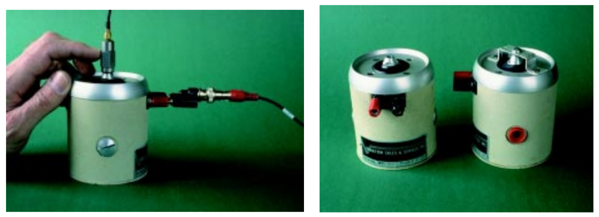
Figure 1 Picture of the LOS model V-203 electrodynamic shaker.
| [1] | Based on the "Down and Dirty" Details of Analog Programming, Sound and Vibration, August 2000 |
Model Description
Figure 2 shows a schematic of the system. The shaker has a compliant suspension of stiffness \(K\) and damping \(C\) suspending a load-table of mass \(M\). The table is driven by a voice-coil of resistance \(R\) and inductance \(L\) which applies a force to the table in proportion to coil current \(i\) by a magnetic constant \(k_2\). The table motion is resisted by the reaction force \(F_r\) of the test object of mass \(M_s\). The moving coil also generates a back EMF in proportion to table velocity and the magnetic constant \(k_1\). The shaker is driven by a voltage \(e_{\textrm{in}}\) from a power amplifier. The test piece mass structure support springs, \(K_s\), have negligible damping.
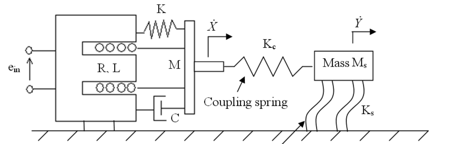
Figure 2 Schematic of the electrodynamic shaker (left side) connected to a test piece (right side) by the coupling spring.
Modify the shaker bond graph shown in Figure 3 to include a coupling spring and a one degree-of-freedom model of the test piece structure shown in the diagram. The reaction force \(F_r\) will now come from the coupling spring (i.e., remove this effort source). On your new bond graph it would make more sense to reverse the direction of the half arrow on the \(F_r\) bond. Turn in a copy of your bond graph including power convention and causal strokes as one of the deliverables.
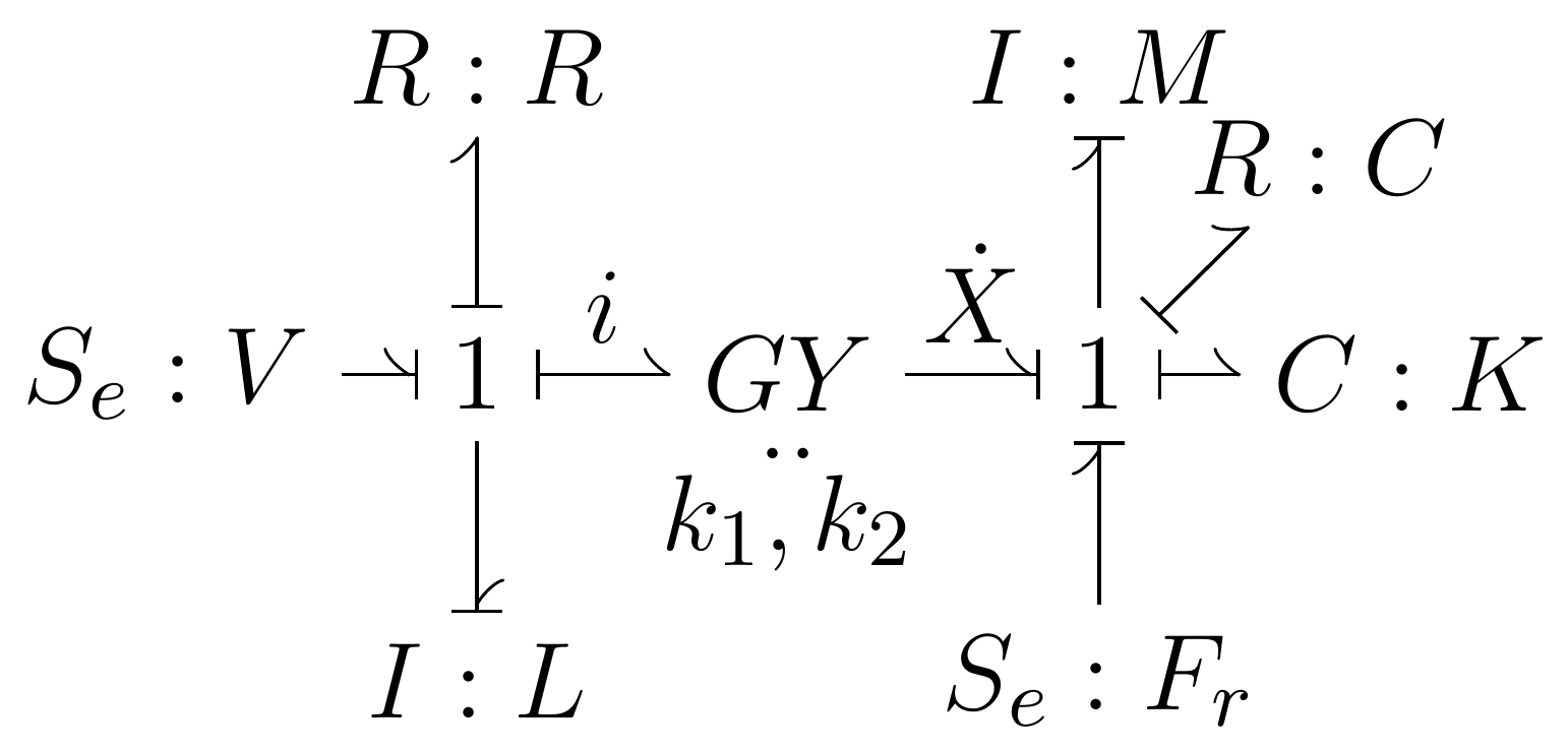
Figure 3 Schematic of the shaker showing key functional elements.
The pertinent equations are from the bond graph in Figure 3 are:
Note that the gyrator with constant \(k_1\), \(k_2\) represents \(e=k_1\dot{X}\) and \(k_2i=F\).
System Equations and State Variables
You will need to arrive at the complete system's ordinary differential equations from the modified bond graph and the provided equations, i.e. replace \(F_r\) with the force generated at the left end of the coupling spring. You will need to determine all of the state variables. Show both the complete differential equations and the list and names of the state variables your report.
Constant Parameters
The basic physics of the system are found in the governing differential equations, and thus you are well on your way to building an analog simulation. However, you need to know all of the coefficients in the equations as well as the expected range of every variable before proceeding. Fortunately, there are some useful numerical values garnered from analyzing it extensively for the Electrodynamic Shaker Fundamentals article mentioned above. In particular, you know:
- \(M_s = 0.7\textrm{ kg}\): mass of the test piece
- \(M=178.04\times10^{-6} \frac{\textrm{lb s}^2}{\textrm{in}}\): shaker table mass
- \(K = 16.54 \textrm{ lb/in}\): shaker internal stiffness
- \(C = 39.09 \times 10^{-3} \frac{\textrm{lb s}}{\textrm{in}}\): shaker internal damping
- \(R = 1.6 \Omega\): shaker coil resistance
- \(L = 764 \mu\textrm{H}\): shaker coil inductance
- \(k_1 = 95.10 \times 10^{-3} \frac{\textrm{V}}{ \textrm{in/s} }\): shaker voltage-velocity proportionality coefficient
- \(k_2 = 0.8416 \frac{lb}{A}\): shaker force-current proportionality coefficient
- \(X_{\textrm{lim}} = \pm 100 \textrm{ mm}\): maximum and minimum shaker stroke
- \(\ddot{X}_{\textrm{lim}}=\pm 135 \textrm{ g}\): maximum and minimum shaker acceleration
- \(F_{\textrm{lim}}=\pm 4.4 \textrm{ lb}\): maximum and minimum shaker force
Buy looking only at the test piece with the shaker is disconnected via the coupling spring, compute a spring constant for the test piece support springs such that the natural frequency, \(f_n\) , of the support structure itself is 20 Hz. Also compute the corresponding compliance (\(C_s = \frac{1}{K_s}\)).
You will need to convert the units given in the handout to the proper SI units used in computation.
Inputs
Using the constants above and the system equations, compute the maximum voltage, \(e_{in}\), that could be applied to the shaker if the force (on the mechanical side of the gyrator) is limited to 4.4 lbs. (Hint: This is a non-dynamic calculation involving only \(k_2\) and \(R\).) Use this as a constant input to the system in your simulation.
Initial Conditions
All initial conditions can be set to zero.
Simulation
First let the coupling spring have a zero or nearly zero spring constant so that the shaker is not affected by the presence of the structure. You can either modify the equation for the spring from the form \(e_c = \frac{q_c}{C_c}\) to \(e_c = K_c q_c\) and set \(K_c\) to zero, or you could use a very large number for \(C_c\).
Use zero initial conditions for all momentum displacement variables and let \(e_{in}\) from your power supply be the voltage you calculated. This corresponds to suddenly turning on the maximum voltage at t = 0.
Simulate the system to see how the shaker behaves on its own. Report on the findings in your deliverables.
Now do two more simulations with finite coupling spring constants (or equivalent compliances). Experiment with the coupling spring constant; try it with values less than the support spring constant and greater than the support spring constant. Be careful of extremely large coupling spring constants, you could create a system which would need a very small step size to be numerically stable. Report on the findings of the two additional simulations in your deliverables.
Time
You have to choose the maximum step size and stop time for the simulation based on the considerations on the shortest period of oscillation or the shortest time constant of the system. You will learn more about these characteristic times of a system in Chapter 6 of the text. Approximates are:
| Oscillation frequency | \(\omega_n = \sqrt{\frac{K}{M}} \frac{\textrm{rad}}{\textrm{sec}}\) |
| Period | \(T = \frac{2\pi}{\omega_n} \textrm{sec}\) |
| Mechanical time constant | \(\tau_1 = \frac{M}{C} \textrm{sec}\) |
| Electrical time constant | \(\tau_2 = \frac{L}{R} \textrm{sec}\) |
The default integration scheme, ode45(), is a variable-step Bogacki-Shampine algorithm (Historical note: Prof. Bogacki taught Prof. Moore calculus in undergrad!). The maximum step size guarantees data points at a regular interval for plotting and analysis. Keep in mind that your max step size must be smaller than the shortest period of oscillation or the shortest time constant of the system. The stop time should be set such that most of the transient response will occur for 0 < t < stop time.
Deliverables
- A bond graph with power conventions, causal strokes, and linear coefficients for all ports.
- Complete system equations and state variables defined.
- A list of all constant parameters in acceptable SI units.
- Show plots of your selected variables for the three cases simulated. Plot at least 4 variables you think would be of interest and explain why they are of interest.
- Explanation of what you observe and learn about the system's motion from the three simulations.
- Append a copy of your Matlab/Octave code to the end of the report.
The report should follow the report template and guidelines.
Code
- Create a function defined in an m-file that evaluates the right hand side of the ODEs, i.e. evaluates the state derivatives. See Defining the State Derivative Function for an explanation.
- Create a function defined in an m-file that calculates any necessary outputs. See Outputs Other Than the States and Outputs Involving State Derivatives for an explanation.
- Create a script in an m-file that utilizes the above functions to simulate the system for three scenarios. This should setup the constants, integrate the dynamics equations, and plot each state, input, and output versus time. See Integrating the State Equations for an explanation.
Assessment Rubric
Points will be added to 40 to get your score from 40-100.
Functions (10 points)
- [10] All functions are present and take correct inputs and produce the expected outputs.
- [5] Most functions are present and mostly take correct inputs and produce the expected outputs
- [0] No functions are present.
Main Script (10 points)
- [10] Constant parameters only defined once in main script(s); Integration produces the correct state, input, and output trajectories; Justified choices in number of time steps and resolution are chosen and explained
- [5] Parameters are defined in multiple places; Integration produces some correct state, input, and output trajectories; Poor choices in number of time steps and resolution are chosen or not explained
- [0] Constants defined redundantly; Integration produces incorrect trajectories; No clear choices in time duration and steps
Explanations (10 points)
- [10] Explanation of dynamics are correct and well explained; Explanation of the vibration period and frequency is correct and well explained; Plots of appropriate variables are used in the explanations
- [5] Explanation of dynamics is somewhat correct and reasonably explained; Explanation of vibration period and frequency is somewhat correctly describes results; Plots of appropriate variables are used in the explanations, but some are missing
- [0] Explanation of damping is incorrect and poorly explained; Explanation of vibration and frequency behavior incorrectly describes results; Plots are not used.
Report and Code Formatting (10 points)
- [10] All axes labeled with units, legible font sizes, informative captions; Functions are documented with docstrings which fully explain the inputs and outputs; Professional, very legible, quality writing; All report format requirements met
- [5] Some axes labeled with units, mostly legible font sizes, less-than-informative captions; Functions have docstrings but the inputs and outputs are not fully explained; Semi-professional, somewhat legible, writing needs improvement; Most report format requirements met
- [0] Axes do not have labels, legible font sizes, or informative captions; Functions do not have docstrings; Report is not professionally written and formatted; Report format requirements are not met
Contributions [10 points]
- [10] Very clear that everyone in the lab group contributed equitably. (e.g. both need to do some coding, both work on bond graph, both should contribute to writing)
- [5] Need to improve the contributions of one or more members
- [0] Clear that everyone is not contributing equitably