Contents
Learning Objectives
After completing this lab you will be able to:
- translate ordinary differential equations into a computer function that evaluates the equations at any given point in time
- numerically integrate ordinary differential equations with Octave/Matlab's ode45
- create complete and legible plots of the resulting input, state, and output trajectories
- create a report with textual explanations and plots of the simulation
- use a simulation to design surge tanks for a hydraulic system
Introduction
Sacramento has built a new hydroelectric power plant. A previous company designed the plant without performing a simulation before the construction. After the plant was completed, and the California monsoonal rains came, the surge tanks could not withstand the dynamics of the flow and the city flooded. Fortunately, the people of Sacramento are great swimmers. Later it was found that the company was staffed with graduates from some junior university from the bay area. The reputation of your fine UC Davis education has gained the confidence of Sacramento's city council, which has refused to pay the bad company, and has hired you to redesign the surge tanks so the town won't have to hire as many lifeguards this spring.
Surge tanks act as hydraulic "springs", absorbing the pressure increase associated with stopping the momentum of the fluid in the pipe. However, because of the reconstruction, our surge tanks must be drilled in stone and this is very expensive for large diameter holes.
Model Description
Figure 1 provides a hydraulic schematic of a reservoir that feeds a hydroelectric turbine. There are two surge tanks that store and release hydraulic energy to help provide a steady flow through the turbine.
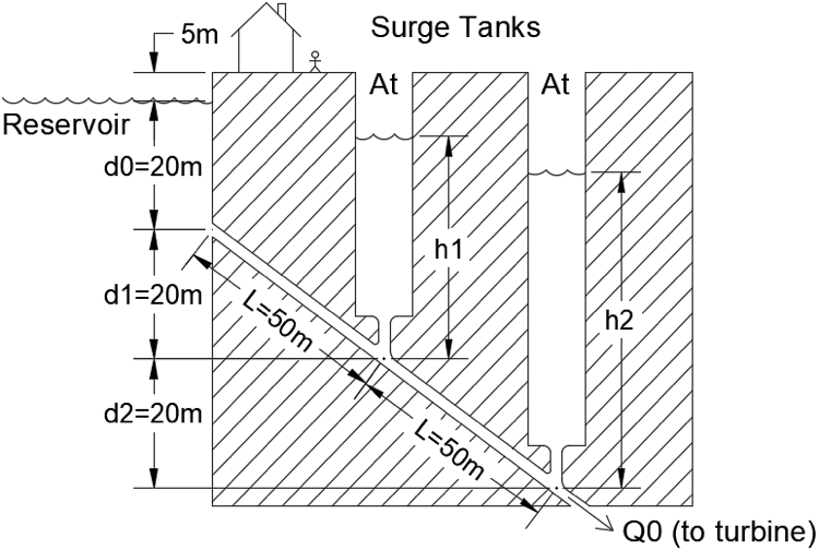
Figure 1 Schematic of the hydroelectric dam with reservoir and surge tanks.
For this system assume that the tank areas \(A_t\) will be significantly larger than the pipe area, \(A_p\), e.g. \(A_t > 5 A_p\), so that there is negligible tank inertia compared to the pipe inertia. Also assume that the tank and reservoir inlets have negligible resistance compared to the pipe resistances.
The bond graph for this system is shown below in figure 2.
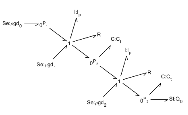
Figure 2 Bond graph of the dam system.
The pipe resistances in this system are nonlinear and behave according to the constitutive law:
which is shown graphically in Figure 3.
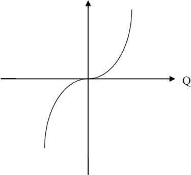
Figure 3 Non-linear resistance constitutive law.
You will need to assign causality to the bond graph, number the bonds, and derive the system equations. You should end up with four differential equations. You will have two fluid momentum state variables (one for each section of the pipe) and two volumetric displacement state variables (one for each tank).
Constant parameters
| Symbol | Description | Value | Units |
|---|---|---|---|
| \(\rho\) | Density of water | 1000 | \(\frac{\textrm{kg}}{\textrm{m}^3}\) |
| \(g\) | Acceleration due to gravity | 9.81 | \(\frac{\textrm{m}}{\textrm{s}^2}\) |
| \(A_p\) | Cross sectional area of the pipe from the reservoir to the turbine | 0.1 | \(\textrm{m}^2\) |
| \(P\) | Hydrostatic pressure (note that the pressure heights between nodes are relative). | \(\rho g \Delta h\) | \(\frac{N}{m^2}\) |
| \(C_f\) | Fluid pipe resistance constant (see figure 3 for \(\Delta P\) vs \(Q\)) | 49000 | \(\frac{kg}{m^7}\) |
| \(L\) | Pipe section lengths | 50 | \(\textrm{m}\) |
| \(I_p\) | Fluid inertia of pipe sections | \(\frac{\rho L}{A_p}\) | \(\frac{kg}{m^4}\) |
| \(A_t\) | Tank areas (you will find the maximum tank area by simulating different values of \(A_t\). Use increments of 0.05 \(\textrm{m}^2\). | To be determined | \(m^2\) |
| \(C_t\) | Fluid capacitance of each tank | \(\frac{A_t}{\rho g}\) | \(\frac{m^5}{N}\) |
Remember that in fluid systems, we use Q for volumetric flow (not displacement) and V as volume (not velocity).
Initial Conditions
Determine the initial conditions from the equations of motion. The system will begin in equilibrium (all state derivatives are equal to zero), with an initial turbine flow of \(Q_0=1.5\frac{\textrm{m}^3}{\textrm{s}}\). You will need to find initial conditions for every state variable. None of the initial conditions will be zero. Develop the initial conditions equations in terms of the system parameters and let Matlab calculate the exact values. Include how you determined the initial conditions in your lab report.
Inputs
Define all system inputs for the effort and flow sources. The effort sources are the pressures due to gravity and are constant with respect to time. The flow source is the turbine flow \(Q_0\). When the turbine is delivering power the steady state flow \(Q_0\) out of the pipe is \(1.5\frac{m^3}{s}\). The turbine flow begins as \(Q_0=1.5\frac{m^3}{s}\) at \(t = 0\). At some time of your choosing, the turbine will begin to turn off. Over the next 0.15 seconds, the turbine shuts down and flow \(Q_0\) decreases linearly to zero. Define \(Q_0\) before, during, and after the shut-down period in an input function file.
Outputs
You will also likely need to take turbine flow (\(Q_0\)) as an extra variable. You may find it useful to define the tank heights as extra outputs as well.
Simulation
Your goal is to find the minimum cross-sectional area of the surge tanks, so that the flow to the turbines can be shut off quickly without overflowing the tanks and drowning the people of Sacramento.
Choose a starting tank area \(A_t\) and simulate the system. Determine the height of the water in the tanks and plot the heights as a function of time. Plot the height of the water in the tank. Increase or decrease the tank area by increments of 0.05 \(\textrm{m}^2\) until you find the smallest possible tank area that does not cause the tanks to overflow when the turbine is shut off Refer to Figure 1 to find the maximum water height in either tank.
Determine your simulation time parameters. In order to gauge how long and what time step to use to simulate the system you will need an idea of the natural frequencies. Since the system is nonlinear, a straight forward frequency analysis is not possible. But since the non-linearity of the system is in the resistance, a rough estimate can be calculated using only the compliance and inertial properties of the system. Here is a hint:
Deliverables
- Show the bond graph with both assigned causality and numbered bonds.
- Show the system equations that you derive from the bond graph.
- Include calculations and explanations for initial conditions, natural frequencies, time parameters, and any other such calculations.
- Plots of the input and tank heights vs. time for the desired tank area (these do not have to be on the same plot).
- Discussion of results
- Which tank came closer to overflowing? Why?
- How do the calculated natural frequencies compare to the vibration periods seen in your plotted results? Why is there a difference?
- Matlab code for the main file, state derivatives, inputs, output functions. Code should follow the best practices form.
The report should follow the report template and guidelines.
Assessment Rubric
Points will be added to 40 to get your score from 40-100.
Functions (10 points)
- [10] All functions are present and take correct inputs and produce the expected outputs.
- [5] Most functions are present and mostly take correct inputs and produce the expected outputs
- [0] No functions are present.
Main Script (10 points)
- [10] Constant parameters only defined once in main script(s); Integration produces the correct state, input, and output trajectories; Justified choices in number of time steps and resolution are chosen and explained
- [5] Parameters are defined in multiple places; Integration produces some correct state, input, and output trajectories; Poor choices in number of time steps and resolution are chosen or not explained
- [0] Constants defined redundantly; Integration produces incorrect trajectories; No clear choices in time duration and steps
Explanations (10 points)
- [10] Explanation of dynamics are correct and well explained; Explanation of the vibration period and frequency is correct and well explained; Plots of appropriate variables are used in the explanations
- [5] Explanation of dynamics is somewhat correct and reasonably explained; Explanation of vibration period and frequency is somewhat correctly describes results; Plots of appropriate variables are used in the explanations, but some are missing
- [0] Explanation of damping is incorrect and poorly explained; Explanation of vibration and frequency behavior incorrectly describes results; Plots are not used.
Report and Code Formatting (10 points)
- [10] All axes labeled with units, legible font sizes, informative captions; Functions are documented with docstrings which fully explain the inputs and outputs; Professional, very legible, quality writing; All report format requirements met
- [5] Some axes labeled with units, mostly legible font sizes, less-than-informative captions; Functions have docstrings but the inputs and outputs are not fully explained; Semi-professional, somewhat legible, writing needs improvement; Most report format requirements met
- [0] Axes do not have labels, legible font sizes, or informative captions; Functions do not have docstrings; Report is not professionally written and formatted; Report format requirements are not met
Contributions [10 points]
- [10] Very clear that everyone in the lab group contributed equitably. (e.g. both need to do some coding, both work on bond graph, both should contribute to writing)
- [5] Need to improve the contributions of one or more members
- [0] Clear that everyone is not contributing equitably