Control
Introduction
I have shown that a basic bicycle model can exhibit stability when linearized about the nominal configuration for a range of speeds, Chapter Bicycle Equations Of Motion. Stability is a strong function of the parameters of the bicycle and it turns out that standard bicycle designs, typically exhibit a speed dependent stability and the bicycle becomes stable at some speed threshold, Chapter Parameter Studies. Based on the damping of the weave mode, one may also even claim that the bicycle becomes more stable as speed increases, neglecting the very slow, easily controllable capsize instability. I’ve also shown that stability can be enhanced or decreased by extending the Whipple model with a flywheel or rider degrees of freedom, Chapter Extensions of the Whipple Model. In Chapter Motion Capture, I’ve examined the kinematics of the rider to see if the rider’s motion during a control task has any correlation to the kinematics of the Whipple model and identified the dominant rider motions during stabilization.
As far as roll stability is concerned, it is highly probable that a human must implement active control at all times while balancing. I conclude this because the bicycle’s roll angle responds to the human’s postural control. But the stability exhibited of the almost-always-present weave mode may alleviate the need for primary roll control provided by the rider. And even if the bicycle-rider system is open loop unstable at a given speed, the question arises of how instable is it or how controllable is it. Classic controllability is simply a binary test to determine whether or not it is possible for a system to be controlled, whereas there must be some measure variable measure of controllability that is more relevant to the proposed questions. [SPC01] studies how parameter changes affect controllability, and comes up with rideability index. [SK10a] and [SMK12] also determine the controllability of several bicycle models and uses modal controllability as a continuous measure of the controllability. The pole locations of an open loop system can also give a general sense of the degree of its controllability, with roots in the far right plane likely being difficult to stabilize.
One can work with different bicycle models (simple/complex [or low/high order] and linear/non-linear), different control structures, and different ways to identify the optimal numerical values for the controller. For a given order model, most control structures allow one to place the closed loop poles in the desired location. Controllers designed for low order or linear models are even likely to work with higher order models and non-linear models. But the control structure design provides different views into the feedback mechanisms at work. For the human controller, these structures may or may not correspond well to the human’s physiological and neurological system. The human has to choose his control actions to balance the requirements for robustness and performance.
The bicycle-rider system presents both a theoretical and experimentally rich dynamical system for control studies. It is very tractable in the sense that most people are familiar with controlling a bicycle and that it is a simple machine which is readily available for experimental use. Additionally, control of the bicycle is not necessarily trivial due to it’s complex dynamics and thus it provides a good platform for testing many control strategies. Past control studies tend to be framed in two different but overlapping frameworks. The first is to simply control a bicycle (model or real) with any control algorithms and mechanisms available. Both the simple roll stabilization task and more complex path tracking tasks have been examined. The results show that bicycles are readily controllable by a variety of means, from a simple steer in the direction of the rate of fall to full state feedback with preview of future path variations. Depending on the sensing and actuation methods chosen these controllers range in their resemblance to how a human may actually control a bicycle. This leads into a second framework in which the researcher is explicitly trying to determine the how a human balances and controls a bicycle. Basic understanding of the limited sensory input and actuation available to a human give constraints on what control structures are adopted. Both frameworks are motivated by many things such as a desire to implement automatic control, improving simulation for vehicle design, handling qualities inquiries, control system testing, etc.
The intention of the work presented in this dissertation falls in the second framework, where we are most concerned with identifying the human controller. The first part of this chapter gives an overview of other non-human based single track vehicle control efforts, followed by some simple control examples. I follow this with a review on human based control design and finish up with some addendum material to our paper [HMH12] which details the controller design we developed to represent the human.
Ideal Control Models
Many studies exist on the control of a single track vehicles. The following provides a light review of much of the literature which focus on ideal controllers for single track vehicles. Here I use the word ideal to simply label control design which is not explicitly focused on the human operator control. I’ve split the review of control models into two sections. The first are about controllers which have actually been implemented, or attempted to be implemented, on robotic vehicles. The second are theoretic controllers that weren’t necessarily introduced to identify the human control system. The following section details efforts that explicitly concern controllers that mimic or try to understand the human controller.
Figure 10.1 shows a histogram by year of the all the references I’ve collected in the course of this project. It is interesting to note the explosion in the early seventies that probably coincides with the bicycle boom and the digital computer age. We’ve also had a boom in the last decade, with research interests growing. This may coincide with the microcontroller advances and potentially some from the growth in bicycling.
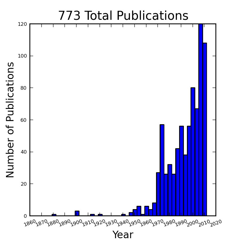
Histogram of my reference database on single track vehicle dynamics, controls, and handling. There are probably 50 or so titles that don’t technically belong, but barring those this gives a good idea of the growth in single track vehicle dynamics research. Generated by src/control/publication_histogram.py.
Robot Control
- [VZ75]
- van Zytveld was one of the first to explore the automatic stabilization of the single track vehicle that was not explicitly in the human control framework, although he did chose feedback variables that he believed a human rider could sense. He attempted to control a robot bicycle with only a leaning rider (inverted pendulum) through proportional and derivative feedback of rider lean angle and bicycle roll angle. He made use of a linear model with a rider lean degree of freedom which is fundamentally the same as the one presented in Chapter Extensions of the Whipple Model. His controller worked on paper, but he wasn’t able to ever balance the robot bicycle, with the suspected problems being the limitations of the hardware he used.
- [Nag83]
- They constructed a robot bicycle which balanced and tracked itself by feeding back lateral deviation at a previewed time and the current roll angle. He was successful at stabilizing his robot. The bicycle model was much simpler than the Whipple model but it gave good agreement between experiment and the model predictions, with the exception of counter-steer predictions.
- [RP85], [RP86]
- Ruijs and Pacejka developed a robotic motorcycle to study the effect of road irregularities (i.e. cat eyes), is this dangerous. The experiments were thought to be to dangerous for a human rider thus the robot was developed. They used a simple control scheme based on gain scheduling as a function of speed. Below the weave speed was lean rate was fed back and above the weave speed lean angle was fed back. Additionally, little bit of steer damping was included. The machine worked as was able to maintain stability during the experiments.
- [BL99]
- They developed a digital fuzzy controller to stabilize a remote controlled bicycle robot. They do not seem to demonstrate the robot actually balancing, but only bench tests of the sensors and actuators.
- [Gal00]
- He designed a robot balancing bicycle which controls a gimbaled gyroscope to apply a restoring torque with respect to the sensed roll angle, but was not successful at balancing the real robot.
- [MKT+01], [MKT+03], [KMBU04], [KKBM05], [MBU+06], [SKK+07]
- These papers, among others, detail work on a Honda motorcycle robot, with the controller modeled after a human. The video demonstrations of this vehicle indicate that it may be the most manually realistically controlled robot there is, not to mention that it seems to work really well. Most of these papers are in Japanese and I’ve had trouble finding others, so I cannot comment on all the details.
- [TM04]
- They successfully balances a bicycle on rollers with a PD roll angle to steer angle controller with a disturbance observer.
- [INM05]
- They use PD control on the bicycle roll angle to control steer angle and rider lean angle. The controller is implemented on a bicycle robot, which is able to balance on rollers.
- [IM06]
- They use the same model base as [INM05] except they now add a human torque estimator, so that the controller will not treat the human’s applied steer torque as a disturbance if the controller is activated while a rider is also trying to control the bicycle. They show some crude experimental results, which I assume are of a rider controlling the bicycle with and without the automatic controller activated. Their human torque accounting is based on an estimation of the human torque from the steer motor torque, rather than explicitly measuring the human’s torque input.
- [YUS06]
- They implement a controller modified from the one presented in [YU05] with an additional \(H_\infty\) controller. They show successful roll stabilization of a robot scooter in which they only implement the roll stabilization control.
- [Mur09]
- The Murata Manufacturing company designed a bicycle robot to demonstrate the utility of their sensors which debuted in 2006 [Mur09]. There is little published detail on the control techniques but they seem to primarily make use of a roll rate gyro with steering and a gyro actuator. They also have other sensors such as ultrasonic sensors for obstacle detection. They demonstrate stability at zero speed, reverse and forward speeds, stopping for obstacles, and tracking a narrow s-curve in their video material. There are no published papers detailing the control system.
- [Tau07]
- This is a Japanese Master’s thesis on acrobatic bike robot that may be able to do a wheelie. I was not able to find this paper but have included it for completeness.
- [MY07]
- They use the same vehicle and control model as in [YUS06] and a new two degree of freedom “rider” pendulum. They demonstrate roll stability of the robot at exactly zero forward and speeds up to 2 m/s.
- [TP08]
- Thanh designs a controller with \(H_2/H_\infty\) techniques and applies it successfully to a bicycle robot which uses a flywheel for stabilization. He compares it to a PD controller and a genetic algorithm and shows that it is more robust.
- [Mut10]
- Mutsaerts designed a Lego NXT bicycle robot with a simple proportional steer into the direction of roll rate controller and demonstrated bicycle roll stability in crude turns and straight ahead running.
- [Bic11]
- In 2011 the first BicyRobo Thailand student competition occurred and many videos on the internet demonstrate the successful design of some teams. The full-size bicycle robots have roll stability and even path following. One video demonstrates students riding the robot bicycle and simultaneously applying manual steer torques.
- [Yam11]
- The videos https://www.youtube.com/watch?v=mT3vfSQePcs and http://ai2001.ifdef.jp/ demonstrate an impressive remote controlled mini robot bicycle that is similar in nature to the [BL99] design with remote control. He uses a commercially available bipedal robot seated on a small bicycle. A gyro detects the roll rate and he uses a PID controller to apply the correct steering for roll stabilization. Remote control is employed to control the heading.
Other relevant papers that I either could not find, translate, or find time to read include [BFG+98], [SS00], [SUK+00], [Mur02], [OMUS02], [MW04], [MT06], [Sup06], [SL07], [TM09], [Bre10], [CALR10], [KY11]. I have included them here for completeness.
The limited success of most of the bicycle robots demonstrates that the actual implementation of single track vehicle control is not trivial. Some robots could demonstrate basic roll stability and some are even capable of path tracking but many didn’t quite work either. The Murata Boy robot is impressive in its abilities but it uses control outside of what humans are capable of. The motorcycle robot by Kageyama et al. is probably the most successful demonstration of a full sized vehicle with control of only steering. The vehicle dynamic models and control methodologies are varied, implying that many techniques may be applicable.
Theoretic Control Models
It is far easier to develop theoretic control models than taking them as far as implementation. There are many more successfully designed models on paper than implemented. This section details some of the modeling efforts.
- [For92]
- He studied the robust stabilization of the wobble mode in motorcycles.
- [Get94], [GM95], [Get95]
- He uses a simple bicycle model that exhibits non-minimum phase behavior and is able to track roll angle and forward velocity using proportional and derivative control. One year later, Getz adds path tracking to his model.
- [KO96]
- He uses a neural network model to balance a two wheeled vehicle.
- [CHA96]
- They use the same simple bicycle model and tracking variables as [Nag83], but controlled it with linear quadratic regulator.
- [Yav97] and [Yav98]
- They study path tracking of a simple bicycle model using some kind of generalized control structure, with a bicycle model similar to [GM95].
- [Sha01]
- They stabilize the roll angle of a motorcycle with a PID controller which operates on the error in roll angle to provide a steer torque. The gains for the controller are chosen by trial and error. The gains are difficult to find for low-speed, high-roll-angle scenarios.
- [STW02]
- They use a simple bicycle model to build a roll rate feedback controller for a high speed recumbent bicycle. They use proportional feedback of the roll rate to control the steer angle.
- [LH02]
- They develop a control model based on something akin to sliding mode control to stabilize the bicycle and track a path.
- [CE03]
- Chidzonga uses the simple point mass bicycle model with a load sharing controller to demonstrate a track stand around zero forward speed. (Although the balancing might have just been due to a miracle from Jesus.)
- [Kar04]
- Karnopp uses a very simple bicycle model and basic proportional control to demonstrate the counter steering require to balance the bicycle. He also examines rear steered bicycles.
- [YU05]
- They set up a linear trajectory tracking control model and non-linear stabilization control by controlling steer torque, rider lean torque, and rear wheel torque. They demonstrate the control in a simulation of a bicycle jump maneuver.
- [NM05b]
- This follows the [TM04] and [INM05] work, but adds velocity tracking.
- [HAP05]
- He makes use of the [CL02] motorcycle model with a eight body rider biomechanical model. He stabilizes the bodies and tracks a path using LQR control.
- [ASKL05]
- They apply simple proportional control of a point mass type bicycle model to stabilize the roll angle with a steer angle input.
- [SN06]
- They stabilize a simple bicycle model using fuzzy control rules to provide a desired roll correction based on the current steer and roll angles. The simulations show stability but with very erratic control that seems like it would be poor for a real controller.
- [LS06]
- They implement a PD controller on roll rate to stabilize the Whipple bicycle model outside the stable speed range.
- [FMPM06]
- A simple point mass bicycle is stabilized with steer angle using three methods: a classical lead/lag compensator design, Ackerman pole placement, and LQR optimal control.
- [Sha07b]
- He develops a path tracking controller for the benchmark bicycle [MPRS07] based on full state feedback and optimal control (LQR). He explores tight to loose control and shows how the gains vary with speed. He also include a preview model of which the tight control needs 2.5s of preview and the loose control needs at least 12.5 s. It is interesting to note that he found little change in computed gains for 20% variations in the various model parameters, leading him to conclude that the rider would be robust to various bicycle designs. His controllers show good performance for randomly generated paths.
- [Sha07a]
- Here Sharp extends his LQR control method with preview from [Sha07b] to the motorcycle with the addition of rider lean torque control. He says that the objective was to develop a control scheme that somewhat represents a rider and which is simple and effective. His controller inputs are the rider’s upper-body absolute and relative lean angles and the path tracking error. He claims that riders control the motorcycle at the weave frequency at high speeds. He is able to successfully stabilize and track a path and determine optimal preview gains. He also finds that the rider lean torque control is relatively ineffective and, even with high weighting in the LQR formulation, the steer torque input dominates the optimal solution.
- [Sha08]
- Sharp applies his LQR based preview model control model from [Sha07a] to the benchmark bicycle. His findings are somewhat similar. His bicycle model is 6th order (he includes heading and path deviation) and he sets up the optimal control problem on full state feedback including varying numbers of path preview points. The bicycle tracks a path well and he shows high, medium, and low authority control by changing the LQR weightings. In general the bicycle roll angle and rate gains are the largest, with rider lean gains following, and steer related gains being the smallest. His leaning rider is initially stabilized by a passive spring and damper, and he finds that the lean torque control is minor when paired with steer torque control. Lean torque alone requires very high gains.
- [MN07]
- Marumo and Nagai design both a PD controller with respect to roll angle and an LQR controller with full state feedback to stabilize the roll of Sharp’s basic motorcycle model through steer torque. The intention is to have a steer-by-wire system so the rider can specify the desired roll angle with something like a joystick, thus alleviating the need for the human to learn to counter steer. They include an additional torque to the controller output computed from the steady state inverse steer torque to roll angle transfer function.
- [CC07]
- Chidzonga expands on the work in [CC07] by once again managing a track stand with a load sharing control scheme.
- [PH08b]
- Peterson designs a yaw rate and rear wheel speed tracking controller based on full state feedback and LQR control. He uses a non-linear Whipple like model with rider lean torque as the only control input. His simulation required 30 Nm of rider lean torque for a 0.3 rad/sec and 1 rad/sec step in yaw rate and rear wheel rate respectively.
- [KM08]
- They stabilize a bicycle model with only a leaning “rider” pendulum actuator and track a path.
- [Con09]
- Connors adds moving legs to the Whipple bicycle model and uses parameters to simulate a low slung recumbent bicycle. He designs an LQR full state feedback controller to stabilize the bicycle.
The following papers were either not found, not translated, or I did not read them, but they all have single track vehicle control: [NII97], [Che00], [PHH01], [FB03], [KN03], [NM05a], [Sac06], [Bje06], [CD06].
Variations on PID control of steer angle or steer torque with feedback of the roll angle are the most popular controller designs, many them being successful. LQR types follow close behind. \(H_\infty\) and other more modern control designs make up the rest. It is clear that roll stabilization and command is the critical task and must be conquered before path tracking can be employed. The steer torque is generally chosen as the primary input with just cause and rider leaning is also used in some models.
Basic Control
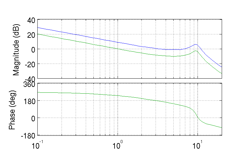
It turns out that the Whipple bicycle model can be stabilized with simple feedback of roll angle or roll rate, with the combination of both working in most cases. [Mut10] in fact demonstrates the simple roll rate feedback stabilization with a small robotic bicycle. But these are not necessarily good controllers, and certainly not controllers which mimic the human. Regardless, their simplicity allows one to demonstrate some of the interesting system dynamics. Take for example Charlie riding on the Rigidcl bicycle at 7 m/s. The linear Whipple model about the nominal configuration gives the steer torque and roll torque inputs to roll and steer angle outputs transfer functions as
The denominators of the transfer functions show that we have three stable modes, as expected. The numerators are potentially more interesting. Note that the steer torque to steer angle and the roll torque to steer angle transfer functions both have a single right half plane zero. This single right half plane zero means that the steer angle response from either input will exhibit an initial undershoot for a given steer torque input [HB07]. This phenomenon can be demonstrated by examining the step response of the two transfer functions with right half plane zeros Figure 10.2.
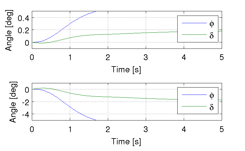
The upper graph shows the roll and steer angle time histories for a step response to roll torque to the Whipple model linearized about the nominal configuration. The lower graph input is for a step input to steer torque. The parameter values are taken from the rider Charlie on the Rigicl bicycle and the speed is 7 m/s which is within the stable speed range. Generated by src/control/control.m.
As expected we see initial undershoot in the steer angle for both cases. In this case, the initial undershoot initially departs in the asymptotic direction, but reverses and settles to a negative steer angle. This is easily demonstrated on a real bicycle by placing one’s flat open palms on the handlebar grips. By applying a torque intending to turn the handlebars in the positive direction, the handlebars initially go in the correct direction, but once the frame rolls in the negative direction, the steering angle reverses and puts the bicycle into a steady turn in the negative direction.
If we examine the change in the transfer function zeros as a function of forward speed Figure 10.3, we see that both the steer angle transfer functions in Equation (1) always have a right half plane zero. And for \(\frac{\delta}{T_\delta}(s)\), the zeros do not change with respect to speed. It is also interesting to note that below about 2 m/s the roll torque to roll angle transfer function has a right half plane zero. For roll torque, this would mean that at low speeds a positive roll torque step input (e.g. a gust of wind[1]) would cause a positive roll angle initial overshoot with the roll angle settling to a negative value at steady state[2].
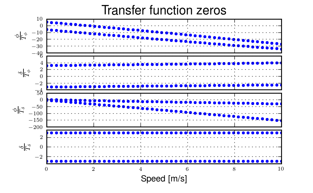
The zeros of the steer torque to roll and steer angle transfer functions. Generated by src/control/zero_wrt_speed.py.
The zeros can be computed analytically with respect to the canonical form presented in [MPRS07].
The state, input and output matrices follow
The numerators of the transfer functions from the inputs to the outputs are computed with
Limiting the solution to only the steer torque input and solving for the roots of the polynomials, the zeros are found
Substituting the benchmark parameters in for the coefficients in Equation (5) which are the zeros of \(\left( \frac{\delta}{T_\delta} \right)_b(s)\) show that they are simply a function of the total potential energy of the system divided by the roll moment of inertia with respect to the center of mass.
This right half plane zero is important for understanding how to control a bicycle. Controlling by steer torque leads to unintuitive behavior of the bicycle, which the rider must learn.
Counter Steering
Countersteering is the colloquial term used to describe the non-minimum phase behavior demonstrated in the previous section. Motorcycle driving instructors are keenly aware of this and teach their students to steer into the obstacle that they want to go around.
[LS06] and [Sha08] explain that the term countersteering is used for two potentially conflicting ideas. They examine the effects of the right half plane zero of a simplified point mass model in much the same way as [ASKL05]. Sharp and Limebeer show that both the steer torque to steer angle and steer torque to lateral deviation have right half plane zeros and Åström develops a steer angle to roll angle transfer function that has a right half plane zero. The Whipple model matches the [LS06] interpretation, i.e. that the right half plane zero is in the steer torque to steer angle transfer function.
The first and most common definition of countersteer is:
To initiate a turn, steer torque is applied in the opposite direction you want to turn which then causes the steer angle to initially depart in the opposite direction of the turn, but after the vehicle rolls the steer angle reverses into the direction of the turn.
The second definition, also clarified by [CLP07], regards the sign of the steer torque in steady turns:
The applied steer torque may reverse sign with respect to the steer angle to maintain steady turn. This is generally true at high speeds.
The step response to steer torque at a stable speed shows that for a given roll angle departure the natural stability enforces that steer angle must initially depart in the opposite direction, Figure 10.2. In the case of roll torque input, a positive roll torque causes a positive roll angle but an initially negative steer angle. Afterwards the bicycle settles into a positive steady turn with respect to yaw. For the steer torque input, a positive steer torque causes an initially positive steer angle which in turn cause a negative roll angle. The bicycle settles into a negative steady turn.
To see this phenomenon outside of the stable speed range some form of control is needed to make simulations stable. Below the weave critical speed, the bicycle can generally be stabilized by a simple feedback gain on roll rate. Note that this gain must be negative, giving positive feedback. This implies that we apply steer torque in the same sense as the rate of fall[3]. Figure 10.4 shows the response to a commanded steer torque below the weave speed under simple control. The countersteering in the steer angle is evident.
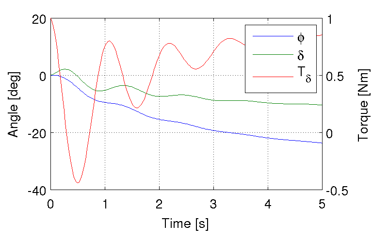
The step response to a commanded steer torque at 5.0 m/s which is below the weave speed. The gain is set to -5. Generated by src/control/control.m.
And above the capsize critical speed, the bicycle can be stabilized by a simple feedback gain on roll angle which also must be negative. Figure 10.5 shows the countering steering required above the stable speed range.
The step response to a commanded roll angle at 10 m/s which is above the capsize speed. The gain is set to -10.1. Generated by src/control/control.m.
For steer torque control inputs countersteering amounts to this: to get the bicycle into a positive turn, one must initially apply a negative steer torque to cause an initially negative steer angle and a positive roll angle. The steer angle exhibits initial undershoot due to the right half plane zero and settles to a positive angle at steady state. This is the case for at least all speeds above very slow speeds where the steer torque to roll angle transfer function has a right half plane zero.
Human Operator Control
There are few studies focusing explicitly on human control of a bicycle or motorcycle with the intent of identifying the human controller or controlling the vehicle with a human-like controller. The majority of the studies of this nature happened in the early seventies when manual control theories were relatively new. The following details the efforts that I’ve come across in my research.
van Lunteren and Stassen
van Lunteren and Stassen did some the earliest work on the subject at Delft University of Technology. They were primarily interested in identifying the human control system in the bicycle riding task. Their studies spanned several years in the late 60’s and early 70’s. [VLS67], [VLS69], [VLS70a], [VLS70b], [SVLB+73], [VLS73] uses a bicycle roll angle feedback with PID control that drives the rider’s lean angle and steer angle. The bicycle model they employ is quite simple (it models their simulator more than a real bicycle) and does not exhibit proper coupling in steer and roll. The model also utilizes angle inputs as opposed to input torques. Their control structure was chosen in part because of equipment limitations but they cite recent manual control models [MGK67a] as being preferable. Nonetheless the research was ground breaking at the time and quite impressive, with real time system identification in a manually controlled electromechanical system. They concluded using roll angle input was more reflexive and that the control using steer angle was more cerebral based on identified time delays. They further developed their system to include a visual tracking outer loop. [DL11] develops a more up-to-date model with the same type of structure as van Lunteren and Stassen, in which he feeds back roll angle and steer angle, and drives steer torque with PID controllers. He also points out a sign error in van Lunteren and Stassen’s work.
CALSPAN
The CALSPAN group developed a controller for their bicycle and motorcycle research that parallels the Delft work except they made use of the latest bicycle and motorcycle models with steer torque and learn torques as plant inputs [RL72]. The specifically point out the advantages of choosing the inputs to be torques and cite the Delft group’s misguided assumptions. They design a PID controller with time delays for both steer torque and rider lean torque control to stabilize the inner roll loop. The outer loops consist of the previewed error in the desired path at several future time steps. This error is weighted to calculate a cumulative error which is then multiplied by a gain to compute an adjustment to the commanded roll angle. They show simulations of both good roll stabilization and slalom path tracking which they compare to video footage of an actual bicycle rider.
Weir and Zellner
Weir worked with McRuer on some manual control papers prior to his PhD thesis [Wei72], where he employed the crossover model together with a motorcycle model which is based on Sharp’s early motorcycle model [Sha71] to evaluate the controller used by humans. This is the first complete attempt at analyzing the rider-motorcycle control system. Weir determined that roll angle feedback combined with a basic human model and a simple gain controlling steer torque was the most descriptive control mechanism. In particular, he showed how steer angle control was poor and he even examined rider lean angle control using a pseudo rider lean model similar to [HMH12]. Rider lean could successfully control the system, but required large lean angles. He also worked with multiple loop closures and found that roll angle fed back to control steer torque, with heading and lateral deviation fed back to control rider lean angle presented the best control strategy for the human rider. He only did his studies at a single high speed with a motorcycle model which only required stabilization of the capsize mode. It is highly likely that these control strategies could vary with speed, especially at low speed where the weave mode is the dominant instability. Weir and Zellner went on to complete several more important studies involving manual control of the motorcycle [WZ78], [WZ79], including a detailed technical report for the U.S. Department of Transportation [WZT79] in which much experimental work was done verifying their mathematical models.
Eaton
Eaton’s PhD thesis builds off of Weir’s work and is primarily focused on validating the Weir models with experiments [Eat73b]. He pairs the successful motorcycle model develop by Sharp [Sha71] with Weir’s McRuer-style manual control models that were based on the crossover model with time delays. He focused on the inner loop roll stabilization tasks. His model uses roll angle feedback and the controller compensates for roll angle error. He eliminates body lean control as an option to simplify things.
Aoki
For completeness, [Aok79] should be included, although I have not had time to study his work. It looks promising with both a human control model and experimental validation.
Doyle
A recently uncovered study by Doyle ([Doy87], [Doy88]), thanks to Google’s book scanning endeavors and Jim Papadopoulos’s persistence in searching, presents a slow speed view for bicycle control in much contrast to the Weir studies, not only because of the speed and vehicle differences, but because it is examined from the view of a psychologist. We engineers are quick to model the human sensory and actuation system, with little understanding of the intricacies of the human brain. Doyle’s treatise gives a refreshing look from outside the engineering box. Doyle’s control model is fundamentally a sequential loop closure with the inner most loop being roll control and the outer two being heading and path deviation. He says that the outer loops are highly dependent on the inner loop. For the inner loop he determines that continuously feeding back both roll acceleration, with integral and proportional gains adjusted by the human as the crossover model dictates, will stabilize the bicycle at non-intended roll angles. To control roll angle, he claims that we do not do this in a continuous way but rather that we apply discrete pulses when the roll angle meets a threshold. The continuous portion of this model has similar form to the one developed by Weir which in turn resembles our model detailed in the next section.
Wu and Liu
I’ll mention briefly some efforts modeling the human with fuzzy control. I have little understanding of fuzzy control but [Clo94] says that fuzzy control methodologies fundamentally let one translate linguistic rules from an expert in controlling the particular system into a control logic algorithm. [TS83] discussed developing fuzzy control rules from the human operator’s actions. This somewhat parallels how the PID controller was developed based on a ship helmsman’s decision structure [Wik12c]. It seems to certainly be valuable for conscious control efforts, but may have deficiencies when trying to determine the control strategy of unconscious control. But a combination of fuzzy logic and crossover type control may prove useful in describing the human control system. Liu and Wu have done extensive work applying fuzzy control to single track vehicles ([LW93], [WL94], [WL95], [WL96a], [WL96d], [WL96b], [WL96c]).
Mammar
[MEH05] developed a motorcycle control scheme based on a motorcycle dynamics model similar to Sharp’s work with steer torque and rider lean angle as the model inputs. He includes a human model with four elements: a simple second order neuromuscular model similar to that of [HMH12], a time delay, gain, and a first order lead filter representing a mental workload model. His control elements include a roll angle feedback gain, a reference signal pre-filter, and a compensator with proportional, integral, and lead control terms. The proportional term in the compensator is the only speed dependent term. They select the numerical values for the control elements using \(H_\infty\) loop shaping for robustness. They finally show simulation results with good performance with regard to disturbance rejection and roll tracking.
de Lange
More recently, [DL11] wrote his master’s thesis on identifying the human controller in the bicycle-rider system. He employed a controller which fed back roll angle and steer angle with PID plus second derivative control and time delays to command steer torque through a neuromuscular model filter to the Whipple model. The model is similar in flavor to van Lunteren and Stassen’s, but more up-to-date and uses more feedback loops. He chose eight gains plus time delays and attempted to identify which loops were not important from the experimental data presented in the next Chapter System Identification. He finds that the critical feedback variables for a stable model were roll angle, roll rate, steering rate, and the integral of the steer angle, claiming the last one is proportional to heading and thus the rider controls heading with steer. He also finds the time delays generally destabilize his model and he removes them.
Hess
Finally, we’ve developed a control model with Ron Hess [HMH12] that is used later this dissertation for human operator identification. The following section gives a brief synopsis, but one should refer to the published paper for more detail.
Conclusion
A single track vehicle can be stabilized and controlled by a variety of means. Controllers based on simplified dynamical models can potentially control more advanced linear and nonlinear models and/or real systems (i.e. steer into the fall). The roll stabilization is the critical task, as path following can’t occur without roll control authority. Few people have demonstrated robust control of a real system which stabilizes in roll at a variety of speeds. Even fewer have added path tracking abilities. It doesn’t seem like anyone has stabilized a robotic bicycle with a controller that has the limitations of a human built in.
Hess Manual Control Model
Many control model architectures can be used to attempt to identify the human control system while riding the bicycle. We are limited by the type of sensory information a human rider can sense, the human’s processing delays, and the bandwidth and physical limitations of the human’s actuators. The human operator has been modeled with simple models like the crossover model, to more complex neuromuscular dynamics, and even fuzzy and optimal control; [Hes97] provides a good overview. Some of the controllers are essentially equivalent placing the closed loop poles in the same place, but make use of different techniques to get to the end result. [DL11] notes that all feedback controllers can be mapped to a common structure. The models may also be different in complexity. But in general, finding the simplest mathematical model capable of capturing the desired dynamics is a good goal. With this in mind, my advisor Ron Hess developed a controller based on the Whipple bicycle model and his previous successful multi-loop human operator models. We present the control model and the loop closure procedure for selecting the five model gains in [HMH12]. This model is fundamentally similar in nature to Weir’s work and is built on the same foundations such as that of McRuer et al. ([MGK67a] [MGK67b]). We similarly found steer angle based control to be troublesome and had success across a broad range of speeds and selection of bicycles with steer torque control. We also employed a similar method of evaluating rider lean control without introducing an extra degree of freedom. It also resembles the work of [Doy87] with the inner loop structure dedicated to roll stabilization and the outer loops to high cognitive control in heading and path tracking.
Basics of manual control theory
Manual control, or human operator control, was primarily birthed from control engineers after World War II. The requirements for machine designs in which humans were the principal control element, such as artillery guns and aircraft, led to human control modeling. Work by [Tus47] theorized early on that human control systems could be modeled similarly to automatic feedback systems. Tustin’s work was followed by years of theoretical and experimental work by McRuer and his group to understand the control system of aircraft pilots.
McRuer’s group found out that humans adjust their control such that the combined human and plant dynamics behave with desirable closed loop dynamics in many types of tracking tasks. This phenomenon can be captured by a variety of theoretical control structures from simple dynamics to complex neuromuscular models [Hes97]. Fortunately, the simpler models can often capture much of the essential dynamics in human-machine systems such as our bicycle-rider system. In particular, we make use of the crossover model [MK74] to structure our controller design. The reason for this is multi-fold. It allows us to use a simple system which has been applied to numerous man-machine systems with good results.
The basic idea of the crossover model is that, when the human is paired with the plant which she is trying to control, the combined open loop transfer function conforms to the dictates of a sound control system design around the crossover frequency [Hes97]. The form of this transfer function for many control tasks remarkably takes the form
The model is governed by only two parameters: the cross over frequency, \(\omega_c\) and the effective time delay, \(\tau_e\). The simplicity of this model and its ability to describe many human in the loop systems is what makes it so powerful.
The model is capable of describing the dynamics of the human at various crossover frequencies and various performance levels. The majority of the model’s experimental validation efforts have been based around laboratory and vehicle control tasks where good performance was required (i.e. skilled subjects).
We also focus only on compensatory control structures where the human closes loops based on output error. This is a simplification as humans are also able to to take advantage of pursuit and preview based control.
Model Description
The control structure was designed to meet these requirements:
- Roll stabilization is the primary task, with path following in the outer loops. The system should be stable in roll before closing the path following loops.
- The input to the bicycle and rider biomechanic model is steer torque.
- The neuromuscular mode of the closed system should have a natural frequency around 10 rad/s to match laboratory tracking tasks of a human operator.
- The system should be simple. In our case only simple gains are needed to stabilize the system and close all the loops.
- We should see evidence of the crossover model in the open loop roll, heading, and lateral deviation loops.
The multi-loop model we use is constructed with a sequential loop closure technique that sets the model up to follow the dictates of the crossover model. The three inner loops manage the roll stabilization task and the outer two loops manage the path following. We include a simple second order model of the human’s open-loop neuromuscular dynamics which produces a steer torque from the steer angle error.
The neuromuscular parameters, \(\zeta_{nm}\) and \(\omega_{nm}\), were chosen as 0.707 and 30 rad/s, respectively, such that the innermost loops gave a typical response for a human operator.
The bicycle is modeled using the Whipple model linearized about the nominal configuration with the primary control input being steer torque. The inner loops are closed with sequential gains starting with the proprioceptive steer angle loop, followed by the vestibular roll rate loop, and the visual roll angle loop[4], Figure 10.6. The steer angle loop in essence captures the force/feel or haptic feedback we use while interacting with the handlebars. The need for this loop is readily apparent when trying to control a bicycle simulation with a joystick or steering wheel with no haptic feedback as demonstrated in [DL11]; the difficultly level is high without it. We found that this proprioceptive loop was essential for stabilization and closed loop performance, unlike typical aircraft control models. The outer loops are also visual: heading and lateral path deviation, Figure 10.7.
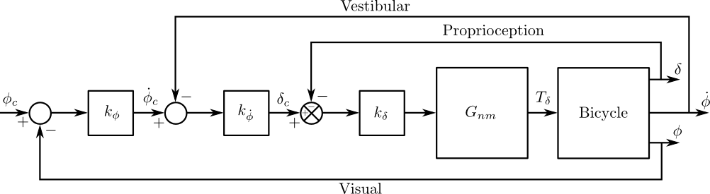
The inner loop structure of the control system with steer angle \(\delta\), roll rate \(\dot{\phi}\), and roll angle \(\phi\) feedback loops.
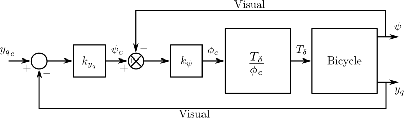
The outer loop structure of the control system with the inner loops closed. The heading \(\psi\) and front wheel lateral deviation \(y_q\) are fed back.
The control structure is simply a function of five gains, which the human “chooses” such that the dictates of the crossover model are met to get good overall system performance. The two inner-most loop gains are chosen such that all of the oscillatory roots of the roll rate closed loop have at least a 0.15 damping ratio. The three outer loop gains are chosen such that the system has a -20 dB slope around crossover. The crossover frequencies are selected sequentially such that the next is half the value of the previous.
Traditionally, sequential loop closure methods are performed on a case by case basis and involve some subjectiveness in applying the design rules of thumb. This is time consuming and error prone when you have to find the gains for many systems such as our bicycles and riders at various speeds. The technique described in [HMH12] can be automated to alleviate this. The following gives the details for developing the gain selection routine.
The roll angle closed loop should be stable, as stability in roll is critical for the path tracking in the outer two loops. To get there, the closure of the proprioceptive and vestibular loops must push the poles to a favorable spot for application of the crossover model on the roll angle loop. To do this, the first two loop closures require that all of the oscillatory modes have a minimum damping ratio of 0.15 and natural frequency around 10 rad/s. We first use the proprioceptive gain, \(k_\delta\) to push the poles originating at the bicycle weave eigenvalue to a higher frequency with about 0.55 damping ratio. The choice of this gain is somewhat arbitrary, but it needs to set the weave mode pole such that it has a small enough damping ratio to allow the roll rate loop to further push it to a damping ratio of 0.15. In [HMH12] we make both loops have a 0.15 damping ratio, but that is not necessary and may not be what the human does. The closed loop transfer function for the steer loop is
where
A numerical example of Charlie on the Rigidcl bicycle at 5 m/s gives numerical values for the open steer angle loop
The characteristic equation is 6th order and the caster, capsize, and neuromuscular modes are all stable whereas the weave mode is unstable. The first loop closure will drive the unstable weave pole out to a higher frequency and mid-range damping ratio.
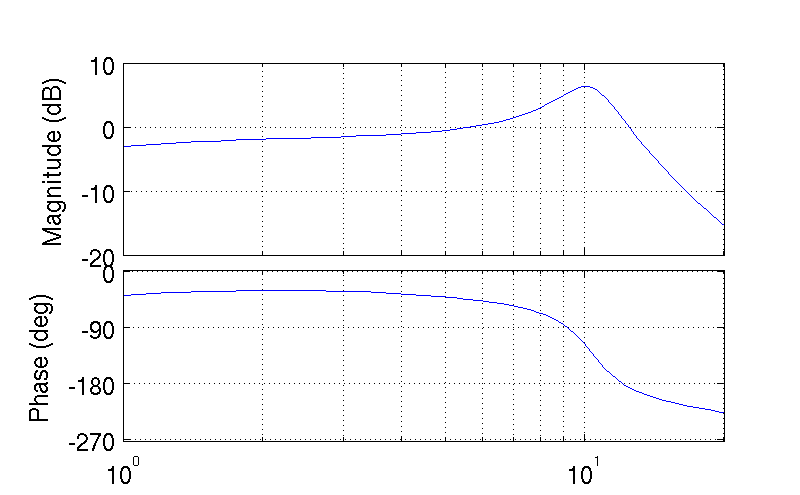
To set the damping ratio multiple approaches can be taken. Here I’ll show a Bode design approach and a root locus based design. For the Bode design we select a gain that creates a damped neuromuscular peak near 10 rad/s, Figure 10.8. For this bicycle and speed, a gain of ~17.5 will set the inner loop as desired.
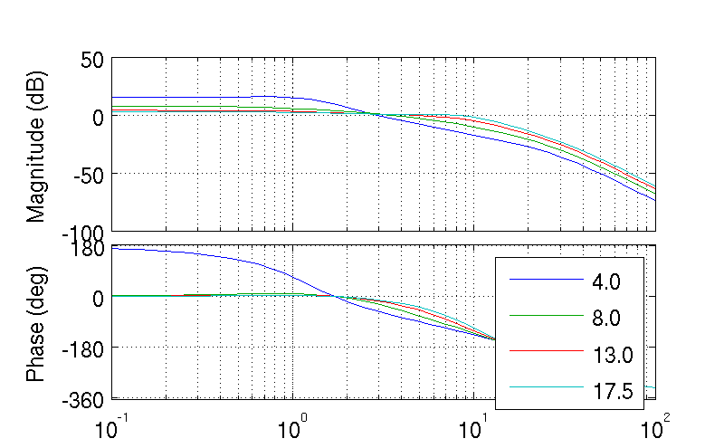
The Bode plots of the closed steer loop with various gains. Notice how the higher gains start to increase the bandwidth by pushing the neuromuscular pole closer to a frequency typical of human operator and plant dynamics [HMH12]. Generated by src/control/choose_gains.m.
By plotting the root locus of the closed loop poles as a function of \(k_\delta\) the desired gain can also easily be picked off on a root locus diagram, Figure 10.9. The root locus of the steer closed loop poles as a function of \(k_\delta\) gives an idea where we can push the poles for the next loop closure. Notice that the poles associated with the weave mode at \(k_\delta=0\) are pushed into the stable regime and back out again, crossing the 0.55 damping ratio line twice. There is a range of gains between about 4.0 and 17.5 which cause all of the oscillatory modes to have at least 0.55 damping ratio. This is very clear when plotting the damping ratio versus gain in Figure 10.10. The best choice typically is to set the gain such that the pole is at the highest frequency allowable with minimum damping, to give typically observed human operator behavior. This will set up the bandwidth of the subsequent loops to be high enough for good system performance.
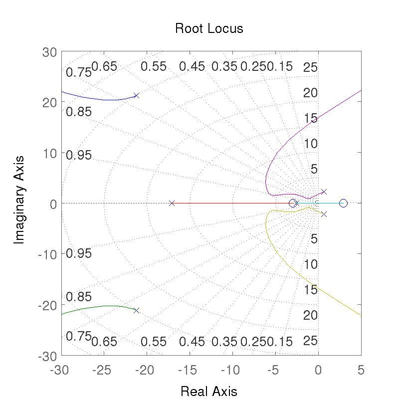
The root locus of the steer closed loop poles versus \(k_\delta\) plotted from 0 to \(\infty\). Generated by src/control/choose_gains.m.
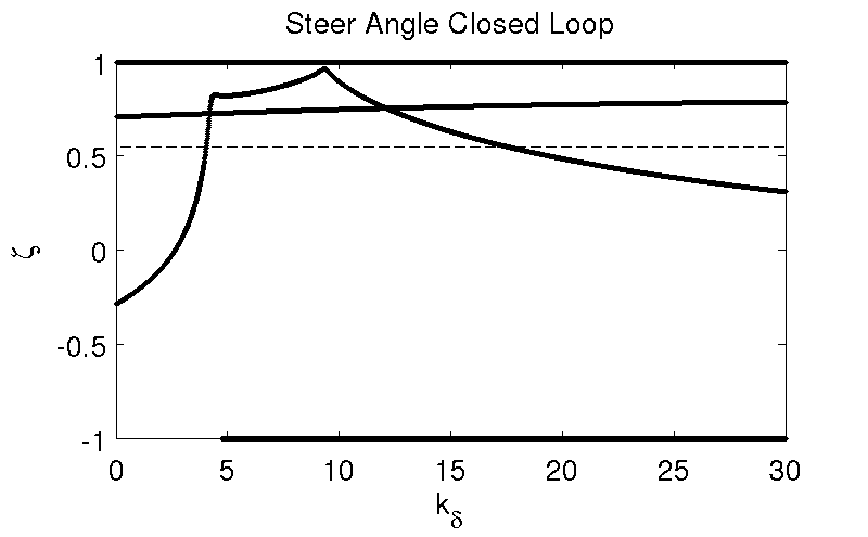
The damping ratio of all the poles as a function of gain. Note that there are gains such that all the roots are stable and the damping ratio is at least 0.55, although inner loop stability is not a requirement for total system stability. Generated by src/control/choose_gains.m.
With the loop closed at \(k_\delta=17.48\) the transfer function takes the form
Notice the single unstable pole at \(s=1.767\). The roll rate loop closure transfer function now takes the form
where
The roll rate loop gain, \(k_{\dot{\phi}}\), is now chosen such that the neuromuscular mode has a minimum damping ratio of 0.15 and frequency is around 10 rad/s. From Figures 10.11 and 10.12 we see that we need to set the roll rate gain to a negative values, about -0.44. Since the bicycle with steer control exhibits non-minimum phase behavior, we need to introduce a positive feedback on roll rate. So it turns out that with a small negative gain we can maintain the neuromuscular mode behavior but introduce the required sign change for stability. This gives the desired 10 dB peaking in the Bode diagram, Figure 10.13.
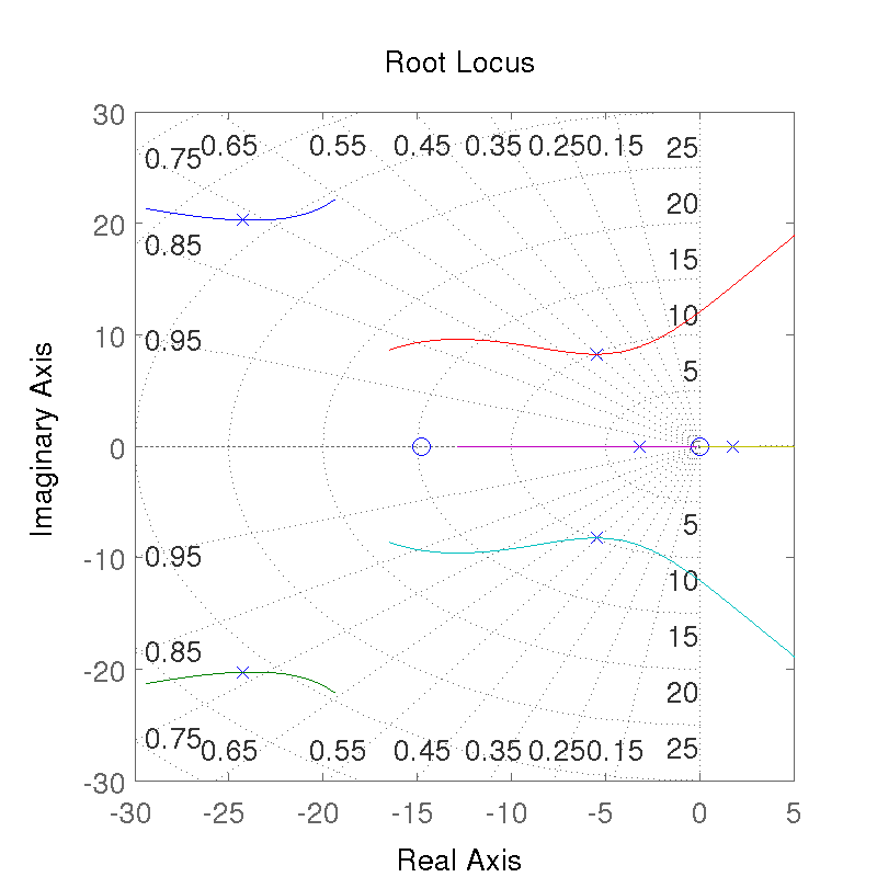
The root locus of the roll rate closed loop for gains \(k_{\dot{\phi}}\) from -4 to 2. Generated by src/control/choose_gains.m.
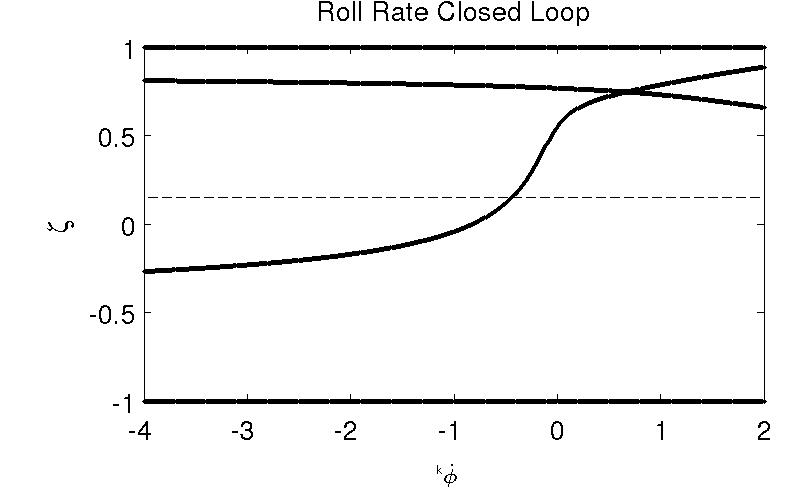
The damping ratio of all roots of the roll rate closed loop as a function of gain \(k_{\dot{\phi}}\). Generated by src/control/choose_gains.m.
The Bode plot of the roll rate closed loop. The neuromuscular mode peaks with a 10 dB magnitude. Generated by src/control/choose_gains.m.
Notice that the closed roll rate loop does not have any right half plane zeros and there is a single unstable pole.
The bicycle-rider system is similar enough in nature for speeds above 2 m/s that this loop closure seems to always work. We’ve had some trouble stabilizing the model at speeds below 2 m/s, with the choice of \(k_\delta\) an important factor in the ability to stabilize at low speeds. [DL11] reported difficulties stabilizing his system below about 2 m/s too. We’ve found that relaxing the 10 dB peak requirement on the inner most loop such that the neuromuscular mode is more damped, will allow for successive closure and a stable system for lower speeds. But as we all know, the bicycle is very difficult for a human to balance at extremely low speeds. The fast time constants compounded with human neuro processing delays makes this true. There are slow bicycle riding competitions that take advantage of this fact to test the balancing skill of the rider.
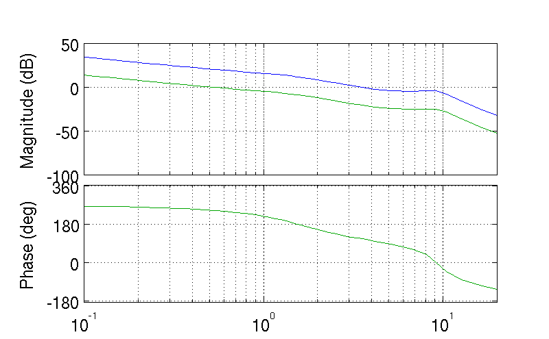
With the roll rate loop closed, the final three loops can be closed by setting the gain such that the crossover frequency of the roll loop is 2 rad/s and the outer loops crossover at half the previous frequency. This is easily set by measuring the gain of transfer function at the desired crossover frequency and realizing that a change in gain will raise or lower the gain curve.
where
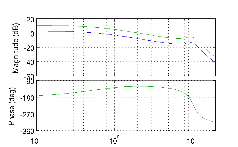
The open loop frequency response for the roll angle loop. Blue is gain of unity and the green line uses the gain to give desired crossover. Generated by src/control/choose_gains.m.
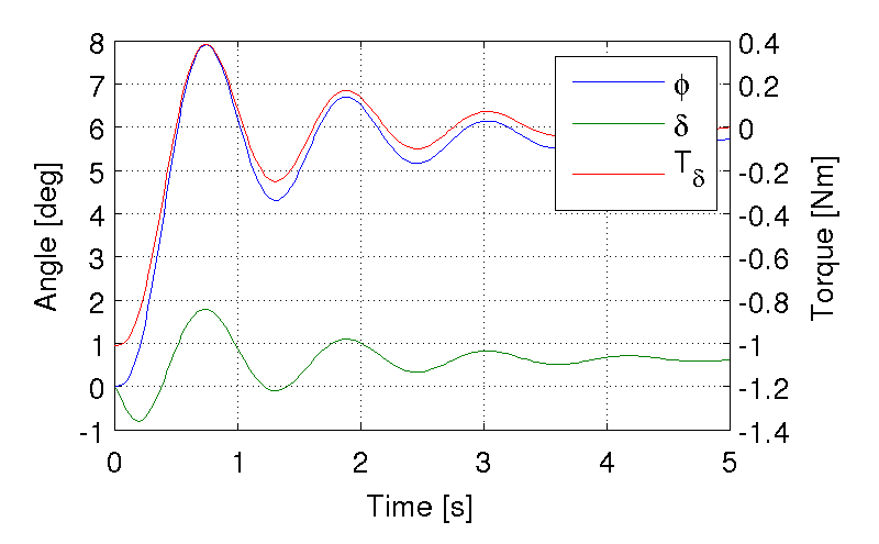
As can be surmised from the Bode diagram, Figure 10.14 we’ve now stabilized the system in roll by forcing the system to behave like the crossover model around the crossover frequency, 2 rad/s. We can now command the roll angle, Figure 10.15.
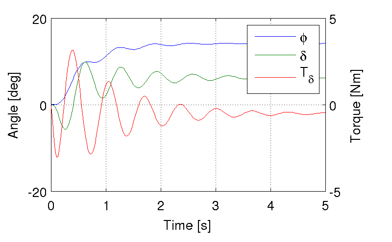
The response of the system for a commanded roll angle of 10 degrees. Notice the initial counter steering and the steady state error in the roll angle. This simulation also demonstrates the steady state negative torque needed for a positive turn. Generated by src/control/choose_gains.m.
It is important to note that this system is a Type 0 system and thus exhibits steady error as seen in Figure 10.15. If we were only concerned with roll stabilization, a low frequency integrator would be needed to remove the steady state error. This was not included in the model design, because the integrator is not needed if the heading loop is closed around the system. The remaining loops are closed using the rule of thumb [Hes97] of crossing over at half the previous inner loop’s crossover frequency.
where
The open loop frequency response for the yaw angle loop. Blue is gain of unity and the green line uses the gain to give desired crossover. Generated by src/control/choose_gains.m.
where
The open loop frequency response for the front wheel lateral deviation loop. Blue is gain of unity and the green line uses the gain to give desired crossover. Generated by src/control/choose_gains.m.
At this point all the loops are closed and the bicycle can track a given path with good performance. The closed loop system bandwidth is approximately equal to the open loop crossover frequency of the lateral deviation loop. Figure 10.18 shows the system response to a step commanded input to lateral deviation.
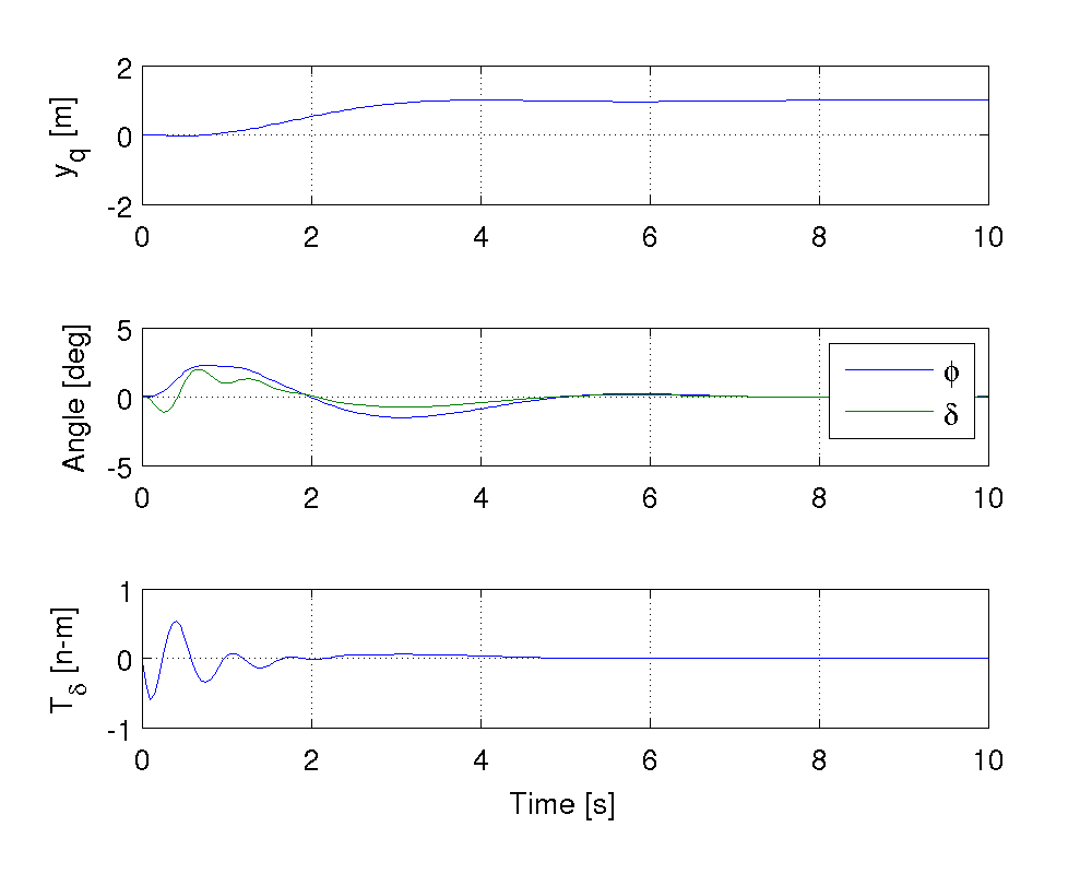
The step response to a commanded lateral path deviation. Notice that for the positive rightward turn, the steer torque and steer angle are negative to initiate the positive turn. Generated by src/control/choose_gains.m.
The gains can be computed across a relevant speed range for the bicycle. We developed an algorithm for automatically selecting the appropriate gains for difference physical parameter values and at different speeds. Figure 10.19 shows how the gains vary with respect to speed for a particular bicycle and rider. Notice that at higher speeds the gains change somewhat linearly, but at speeds below 3 m/s there is non-linear variation. These gains give stable systems which are capable of the lane change maneuver but, due to the difficulties in selecting the gains with the rules above, the algorithm may be making poor choices, especially for \(k_{\dot{\phi}}\), at very low speeds.
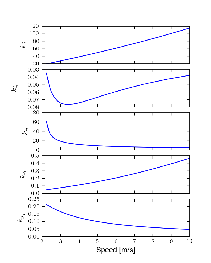
The auto computed gains as a function of speed for the Whipple model with the parameter values from the Davis instrumented bicycle with Jason as the rider. These gains were computed with the method in [HMH12]. Generated by src/davisbicycle/plot_gains.py.
We automated this method based on the Bode design guidelines. The gain choices for proper neuromuscular peaks in the inner most loops require good initial guesses, as there are often multiple solutions. The correct solution puts the neuromuscular natural frequency at a typical value for human operators.
Software
We designed a software suite in Matlab to implement the automated gain selected for various bicycles, riders, and speeds. The software was constructed around a Simulink version of the model described above and offers this functionality:
- It generates the state space form of the linear Whipple model for any parameter sets and speeds. The outputs include all eight of the configuration variables and their derivatives reported in Chapter Bicycle Equations Of Motion with the addition of the front contact point. This includes the lateral force input described in Chapter Extensions of the Whipple Model.
- It generates the state space form of the closed loops system as a function of the bicycle-rider parameters, the speed, the five gains and the neuromuscular frequency.
- It computes the gains with the sequential loop closure guidelines described above for any give bicycle-rider and speed. (Very low speeds may require some manual tweaking.) The open and closed loop transfer functions for each loop can be returned and or plotted. It can also do this for roll torque as the input as described in [HMH12].
- It simulates the system performing a single or double lane change with a given or computed set of gains and plots the results.
- It computes the lateral force input transfer functions.
- It computes the handling quality metric described in [HMH12].
- It plots the gains versus speed.
The software was used to generate most of the results and plots in [HMH12] and the source code for doing so is included. The source can be downloaded at https://github.com/moorepants/HumanControl.
Notation
- \(T_\delta\)
- Steer torque.
- \(T_\phi\)
- Roll torque.
- \(M,C_1,K_0,K_2\)
- The velocity and gravity independent canonical matrices of the Whipple model.
- \(\mathbf{0}_{n \times n}\)
- An \(n \times n\) matrix of zeros.
- \(\mathbf{I}_n\)
- An \(n \times n\) identity matrix.
- \(v\)
- Forward speed.
- \(g\)
- Acceleration due to gravity.
- \(\mathbf{A},\mathbf{B},\mathbf{C}\)
- The state, input, and output matrices.
- \(s\)
- The Laplace variable.
- \(s_\phi,s_\delta\)
- Roots of the steer torque to roll angle and steer torque to steer angle transfer functions.
- \(m_T\)
- The total mass of the bicycle-rider system.
- \(z_T\)
- The height of the center of mass of the total bicycle-rider system.
- \({I_T}_{xx}\)
- The moment of inertia of the bicycle-rider system about the longitudinal axis.
- \(G_{nm}(s)\)
- The neuromuscular transfer function.
- \(\zeta_{nm}\)
- The neuromuscular damping ratio.
- \(\omega_{nm}\)
- The neuromuscular natural frequency.
- \(k_{\delta,\dot{\phi},\phi,\psi,y_q}\)
- The controller loop gains.
- \(x_p,y_p\)
- Rear wheel contact point.
- \(x_q,y_q\)
- Front wheel contact point.
- \(\psi\)
- Yaw angle.
- \(\phi\)
- Roll angle.
- \(\delta\)
- Steer angle.
- \(G_{xo}(s)\)
- The open loop transfer function of loop \(x\).
- \(G_{xc}(s)\)
- The closed loop transfer function of loop \(x\).
Footnotes
| [1] | A gust of wind does not impart a pure roll torque. The wind acts on both the front and rear frames and the rider. Pure roll torques that map to the input described in Chapter Bicycle Equations Of Motion are not necessarily observable in nature. |
| [2] | I’ve often felt like I fall into the wind on my bicycle and this could confirm it at least for low speeds, but it may be tied more to phenomena associated with the rider’s biomechanical degrees of freedom. |
| [3] | The system can be stabilized by negative roll angle feedback at speeds close to the weave critical speed. |
| [4] | [Doy88] notes that his riders can balance even while blindfolded. This is even true for people who’ve been blind since birth. So the roll angle dectection, must necessarily not be all visually based. Indeed, in aircraft flight control, the so-called vestibular “tilt-cue” (the human’s ability to effectively sense roll angle, \(\phi\)) is a well-known phenonmenon, e.g., [JMJ78]. |
