System Identification
Preface
I started to think about system identification when I arrived at Delft and the discussions began with Arend and Jodi. I hadn’t much clue about the formal field and theory of system identification. My first look at it was when Arend presented me with a light introduction by Ljung, so I credit Arend and his cohorts for the ideas that have been implemented in this chapter. We talked about it here and there but never really put together a solid experimental plan to do anything about it. Karl Åström visited us in Delft in late 2008 and we talked some with him about system identification of the bicycle. I mainly recall him focusing on how to excite the system in a very controlled manner with an oscillating mass on the bicycle. Some of these ideas propagated through Arend to Peter and can be seen in the final sections of his thesis [DL11]. Many of these ideas influenced our NSF proposal and ultimately the final portion of what I was to do for my dissertation work.
Once I had gotten back to Davis we now had the resources available from NSF funding to make something happen. My goal had basically formalized into creating a instrumented bicycle to be controlled by a person that was capable of measuring all of the kinematics and kinetics involved in regulated control tasks. We also originally had hoped to be able to vary the dynamics of the bicycle, but the reduced funding nixed that idea. It took some time into the project to really understand what we might be able to accomplish with that but it finally materialized into validating Ron’s theoretic control model which is discussed in [HMH12] and Chapter Control with data collected via the instrumented bicycle. After our first experiments, over a year into the project timeline it became apparent that simple tasks with measured lateral perturbations would provide the best chance of validating his model. Unfortunately, I had not thought a great deal about how to provide and measure these lateral perturbations but the manually excited perturbations seemed to do the trick.
We ran a lot of preliminary system identification analyses on the first set of trial data, but it quickly became apparent that we had little understanding of the subject. The early analyses did give confidence that the data was of good enough quality to do something with, but our goal of identifying the parameters of the controller were still far from our reach.
We performed the final set of experiments around August and September of 2011 to get a large sample of data for the final analyses. The NSF grant was to end at the end of September and I still had to figure out how to analyze all of the data, not to mention write up a ton of work for my dissertation. We ended up extending the NSF grant another year (as seems to be typical with these things). I look back to our original proposal and in hindsight the scope was way too large (accurately predicted by Arend). We nixed the handling qualities parts when the funding was lowered, but I now see that what we hoped to do really took another 6-12 months longer than we had intended.
The final analyses have forced me to figure out what system identification is all about and I’ve learned a great deal rapidly and much on my own. At this stage we weren’t able to find any local experts on the subject to help us along but I’ve gotten some great insight from both the single track vehicle dynamics email list and from personal communication with Karl Åström. I still feel very weak in the subject but it is more clear how difficult identifying complex systems is, especially trying to nail down physical parameters.
As many doctoral students probably hope when starting their long trek to the PhD, I hoped for some grand findings to arise from this work. But I’ve been humbled a lot in that quest. I present here the work I’ve done with regards to identifying the bicycle and rider system with what I think are good results, but I hope that it can be a guide for others to see some of the difficulties in executing this kind of analysis with some ideas to better structure it.
Introduction
The work presented in this Chapter is intended to be the icing on the cake that takes into account all of the theory presented in the previous chapters and evaluates it with a large set of data taken with the instrumented bicycle described in Chapter Davis Instrumented Bicycle. It is also the overarching deliverable I was responsible for under the NSF grant. This chapter details system identification of a bicycle and rider system. It is broken in two main parts, the first goal being to identify the passive bicycle rider system and the second to identify the active portion, i.e. the rider’s control system. The literature review gives an introduction to other’s efforts in both these analyses with respect to single track vehicles.
Two important concepts need to be mentioned briefly before proceeding. The first is a review of the terms used to categorize model structures in the system identification field: white box, black box, and grey box. System identification is the process of identifying a model that best predicts a particular input/output relationship. If we develop a model entirely from first principles[1], e.g. using Newton’s laws to describe the motion of an object, when all of the parameters and states are known then this is called a white box model because we know everything about it a priori. The second case, the black box model, describes a model in which one only knows the structure, i.e. order, of the underlying equations but all the coefficients are unknown. Finally, the grey box model falls in between the first two in that one may have more knowledge of the structure of the coefficients based on first principles, e.g. one may know that some model coefficients are zero or that the model may be parameterized by some known and some unknown physical characteristics.
The second concept regards the notion of process and measurement noise in a dynamic system. Dynamic systems have states that evolve dynamically through time, but a real system has elements that are not purely deterministic which are typically called noise. The noise can be broken up into the process noise, the noise due to errors in, or random inputs into, the model, and the measurement noise, the noise due to errors in the measurements. The ability to characterize these two types of noise plays a large role in the accurate identification of dynamic systems.
Literature
There is a rich history of bicycle and motorcycle mathematical model development. This has been able to explain many of the more dynamically fascinating phenomena, from countersteering and stability to speedman’s wobble and gyroscopic effects. But the amount of experimental validation of these idealized models pales in comparison, with the motorcycle experimentation outdistancing that done with bicycles.
Basic bicycle and motorcycle identification is typically done on data collected by exciting the vehicle through force/torque perturbations in either roll or steer. These experiments can be done when the bicycle is under closed loop control or when the bicycle is stable, the former being a requirement for speeds outside of the stable speed range. But, the mode excitation methods are limited to the frequency band around that mode of motion. Manual excitation under closed loop control gives better excitation bandwidth and a pairing with modern system identification techniques can provide richer models.
Passive Vehicle and Rider Identification
Identification of passive, open loop vehicle-rider models is more prevalent than the identification of the controller. It is indeed a requirement to have a very good vehicle model before attempting to identify the control system a human employs while controlling the system. The bicycle and motorcycle are excellent choices for manual control experiment design due to the fact that they are relatively economical systems that require a broad range of human control skills to stabilize and direct the vehicle, but they have the disadvantage that first principles models are somewhat more difficult to develop and have smaller pool of prior research as say cars or aircraft. The approaches to identifying the passive model include mode excitation techniques to system identification under more general inputs.
CALSPAN
The earliest comprehensive bicycle model validation began at CALSPAN in the late 60’s. This included several revolutionary studies, in one of which they made use of a rocket to apply know step torques to an uncontrolled riderless bicycle. In another, simulations of slalom maneuvers were visually compared with video footage [RM71].
Eaton
David Eaton’s work ([Eat73b], [Eat73a], [ES73]) may be the closest example to the work presented in this chapter. He did his PhD work at the University of Michigan under the Highway Safety Research Institute. His dissertation focused on the experimental validation of the motorcycle modeling work of [Sha71] and the human controller modeling work of [Wei72]. He did this with two sets of experiments: 1) identification of the uncontrolled dynamics of the motorcycle under perturbations, and 2) identification of the rider controller during roll stabilization tasks. The latter of which will be discussed in the next section.
His initial experiments were aimed at validating and identifying the passive motorcycle system. During these experiments, his subjects road a motorcycle with their bodies rigidly braced to the frame and hands-free at speeds of 15, 30, and 45 mph (6.7, 13.4, and 20.1 m/s) along side a pace car which recorded the output from roll angle, roll rate, and steer angle sensors. The brace and open loop response allowed rigid rider modeling assumptions to be used. Weights were dropped from one side of the motorcycle to induce a step roll torque and the rider used a single pulse in steering torque to the handlebars to right the motorcycle in roll after the drop. These experiments were impressively dangerous and would be hard pressed for approval by the Institutional Review Board if done today, but well designed for the typical modeling assumptions. The resulting time histories of the measured system outputs were compared to simulations of Sharp’s model [Sha71] augmented with a variety of tire models of Eaton’s design. He found good agreement between the experiments and the models for higher speeds, but felt that a more complex tire model was needed to predict the wobble mode in slower speed runs.
The second set of experiments were more tame. The three riders simply balanced the motorcycle on a straight path at two speeds, 15 mph and 30 mph, for a total of 38 runs. He added a steer torque transducer bar above the handlebars. The rider controlled the motorcycle with one hand and the rider applied torque was recorded along with the other signals. No perturbations were necessary, as the rider’s natural control actions excited the system in a wide enough bandwidth. From this data he was able to identify the motorcycle steer torque to roll angle transfer function through the spectral densities of the measured signals (by dividing the cross spectrum of the roll angle and steer torque signal by the power spectrum of the steer torque). The identified transfer functions show good agreement with the augmented Sharp motorcycle model at the 30 mph speeds, but less so for the 15 mph runs.
His generated frequency responses from the second experiments provided an empirical model, while the simulation comparisons from the first experiments were validation rather than identification.
Weir, Zellner, Teper
Weir, Zellner, and Teper performed an extensive experimental study on motorcycle handling qualities for the U.S. National Highway Traffic Safety Administration in the late 70’s, [WZT79]. This was a follow up to both the CALSPAN studies and [Tag75], both under or related to the same Administration. There is little to no explicit system identification in the study but some important elements are there. In terms of the passive model identification, they present steady state comparisons of their experimental data to their models with varying degrees of qualitative agreement and generally good ability to predict the conditions at which sign reversals in torque are needed to maintain a steady turn. They also compare single lane change simulations of a controlled vehicle to their measured data by visual inspection. They unfortunately admit that adjusting the first principles models to better fit their measured data was outside the scope of the project. But this gives some early examples of model evaluation with respect to good quality data.
James
Stephen James published a study in 2002 [Jam02] in which he attempted to identify the linear dynamics of an off-road motorcycle. He measured steering torque, steer angle, speed, roll rate, and yaw rate with his subjects manually exciting the vehicle through steer torque during runs at various speeds on a straight single lane road. He made use of black box ARX SIMO identification routines of 6th and 7th order (his and others motorcycles models are usually 10th+ order) to tease out the weave and wobble eigenvalues. He compares the identified eigenvalues, eigenvectors and frequency responses to his motorcycle model and claims good fits based on visual interpretation of the plots. The agreement is questionable due to the lack of statistics in the model comparisons and little validation of his first principles model which assumes a rigid rider. The study does show that there is the possibility of identification of multiple modes of motion with simple manual excitation of the handlebars. He also used these techniques to identify the same motorbike with a single wheel trailer in [Jam05].
Biral et al.
[BBCL03] performed a nice study to identify motorcycle dynamics under an oscillatory steer torque input. They measured steer torque, roll rate, steer angle, and yaw rate with an instrumented motorcycle. They performed slalom maneuvers at speeds from 2 to 30 m/s at three sets of cone spacings in the slalom course. The resulting time histories were close to ideal sinusoids. They used curve fitting to find amplitude and phase relationships among the measured signals. The results were plotted on Bode plots for comparison to the frequency response of several first principles models. The models predict the experimental data and their motorcycle model is shown to do a better job than other models from literature. This claim is only based on visual inspection. I would say this technique and others like it are more of an ad hoc method of system identification of the vehicle dynamics because they rely heavily on very specific input and output characteristics, but nevertheless seems to be effective. Making use of formal system identification techniques could potentially give more reliable results and the ability to better characterize the uncertainty in the predictions.
Kooijman
Jodi Kooijman has worked on experimental validation of the benchmark bicycle [MPRS07] linear equations of motion for a riderless bicycle [Koo06], [KSM08], [KS09]. His instrumented bicycle measured the steer angle, forward speed, roll rate, and yaw rate. Due to the fact that the bicycle can be stable at certain speeds he was able to launch the bicycle in and around the stable speed range and perturb the bicycle with a lateral unmeasured impulse and record the stable decay in the steer, roll, and yaw rates. The post perturbation time histories of the measured signals provided nice decaying oscillations and curves could be fit to find both the time decay constant and frequency of oscillation. These were then compared to the predicted weave response based on the first principle model numerically populated with measured physical parameters of the bicycle. He found good prediction abilities of the weave mode between 4 and 6 m/s. The “goodness” of fit were gaged by visual inspection with no uncertainty estimates in the models or the results from the dynamic measurements. The method was not able to predict the heavily damped caster mode nor the capsize mode. He also demonstrated that the measured dynamics were the same when the experiments were performed on a treadmill.
In [KMP+11], Jodi constructed a bicycle with very unusual physical characteristics including negative trail and canceled angular momentum of the wheels. He performed similar experiments to his Master’s thesis work. They show the comparison of a single stable experiment in which yaw and roll rates were measured and compared to the predictions of the benchmark bicycle.
[Ste09] and [ER11] both perform experiments similar to Kooijman’s with similar results, although Steven’s results vary in the ability of the model to predict the data for various configurations of his adjustable bicycle.
These also fall into the ad hoc system identification techniques that take advantage of the stability at certain speeds and very specific output characteristics. The variability in reproducibility in the studies from other researchers should be noted.
Chen and Doa
[CD10] develop a first principles non-linear bicycle model with a fuzzy controller and use it to generate stable simulations for various speeds. They then do an output error grey box identification on the resulting data with respect to the non-zero and non-unity entries of the state, input and output matrices (i.e. just the entries of the acceleration equations). The identification is done for a discrete number of speeds in the range 1 to 15 m/s. The eigenvalues are calculated of the resulting identified, speed-dependent A matrices and the root locus plotted versus speed.
The resulting eigenvalues seem to behave like the benchmark bicycle but the capsize mode is shown to go unstable briefly at a speed lower than the stable speed range. They did not attempt to characterize or identify the process noise even though they generated the data with a known model with known input noise. Also their non-linear bicycle equations of motion [CD06] were never validated against any other accepted models. Both of these could potentially explain the discrepancies in their identification. Their identification procedure does show that it may be possible to get good estimates of a linear model of the vehicle alone from noisy data regardless of the controller which stabilizes the vehicle.
Doria
In [DFT12] experiments are performed where a motorcycle rider excites the steering with a pulse and lets the motorcycle oscillate while the rider keeps his hands on the handlebars (as opposed to Eaton’s hands-free experiments). The resulting dynamical measurements are nice decaying sinusoidal-like motions and the authors fit optimal curves to the data. They identify the time constants, and frequency and phase information to construct the eigenvalues and eigenvectors of the excited mode. The empirically derived eigenvectors show some resemblance to the model’s predictions.
Controller Identification
van Lunteren and Stassen
At Delft University of Technology in the Man-Machines research group, Drs. van Lunteren and Stassen began work in 1962 to identify the human controller for a normal population of subjects and report on their work into the early 70’s ([VLS67], [VLS69], [Sta69], [VLS70a], [VLS70b], [VLS70c], [VLS73], [SVLB+73]). They chose a bicycle simulator as the plant because it was a common task that average people could do and their studies could focus on a wider population of individuals as compared to most previous work based around trained pilots. The bicycle simulator did not capture all of the essential dynamics of a real bicycle as it’s operation was based on only the simplified roll dynamics of Whipple’s model, but nonetheless offered a similarly complex roll stabilization control task as a normal bicycle would. The simulator was controlled by both the steering angle and the rider’s lean angle, both of which are questionable inputs as have been pointed out as early as [RL72].
They assumed the rider’s control actions can be described by a PID controller with time delays on each feedback variable and mention that this controller was chosen instead of a McRuer style controller primarily due to limitations of their computational equipment. The error in the roll angle is fed into two PID controllers each with a time delay: one to output the corrective steer angle and the other to output the corrective lean angle. They introduce a remnant term for each control action and the external disturbances to the bicycle model.
The identification goal was to find the six gains and two time delays in which the controller performed as a human would. The preferred method was a real time estimation routine due to the speed of computations and reasonable agreement their correlation method. The results indicated that the subjects used no integral control (i.e. only position and rate feedback). They could identify within a bandwidth of about 2 Hz and noticed that when the system was undisturbed there was a 0.5 Hz dominant frequency in the rider’s control actions. The rate feedback was more dominant in generating the lean control input than it was for the steer control input. Also, they found the time delay for lean to be larger than the steer time delay and postulate that the steer action is a result of cerebral activity while the lean is more of a reflexive pattern. Another finding resulting from analysis of Nyquist plots of different riders’ identified control actions showed that riders chose different control actions. They attribute this to the roll stabilization being a sub-critical task (i.e. a more difficult task may force different riders to adopt similar control behavior). They also investigated the effects of drugs, such as alcohol, on the riders control behavior. They found correlations from drug dose to time delays and the error in the control actions. Their later studies introduced better identification methods and they found discrepancies in the identified time delays of the later work as compared to the previous work. For example, the steer control time delay was originally found to be around 1.5 seconds and the improved methods found the delay to be around 0.7 seconds. The discrepancy was attributed to the bias due to remnant in their early work. They also introduced a visual tracking task into the simulator but had difficulties in getting reliable transfer function identification as compared to the roll stabilization transfer functions which improved in quality due to longer trials of 35 minutes.
The methods developed in their studies are excellent and thorough examples of early parameter identification in human control tasks. The simpler plant dynamics were most likely beneficial in reducing the uncertainty in the identified parameters, but the choice of angles as inputs instead forces of torques may not be a realistic enough model of the human’s actuation.
Eaton
After feeling confident in his motorcycle identification results, Eaton made use of the Wingrove-Edwards ([WE68], [WEC69], [Win71], [Edw72]) method in tandem with an impulse identification to identify the human controller. The remnant element was large with respect to the torque that was linearly correlated with the roll angle, but the human control element was identified with a simple gain and time delay for most of the high speed runs. The time delay identification of about 0.3 seconds was very repeatable across all runs. Furthermore, he demonstrated that the crossover model was evident in the resulting closed loop rider-motorcycle transfer functions.
Eaton is one of very few who have identified the rider controller during actual single track vehicle tests with confidence in the underlying passive rider-vehicle model. This study has influenced the work in this chapter in many ways.
Doyle
A recently uncovered study on the manual control of a bicycle from a psychologist’s perspective has some very non-traditional techniques and outlooks for the understanding of the control system employed while balancing a bicycle [Doy87]. Anthony Doyle’s paper [Doy88] on his thesis topic opens with “The old saw says that once learned it is never forgotten, but what exactly is learned has been by no means clear.” This reflection points to the great complexity behind balancing a bicycle, such an easily gained skill. He chooses to study the bicycle over a simpler task partially due to the fact that the rider has little freedom in effective control strategies and partially because it is a skill many people can do.
His goal was to determine how much of the rider’s control actions can be accounted for without involving higher cerebral functions. He mentions the Weir and Zellner work and the fact that its focus is on motorcycles at high speed, and questions whether the control employed for their system is simply a different version of the one employed on a bicycle at low speed or whether they are different control methodologies altogether.
He was aware of the inherent stability that bicycles can provide and constructs an instrumented bicycle where the head angle, trail, and front wheel gyro effects are eliminated so that “all steer movements are a result of the human’s control”. He also mentions, but doesn’t use, a body brace to eliminate unnecessary body movements and he blindfolds his subjects so that their sensory information is limited to proprioception and vestibular cues. He mentions the arm and upper body movements and how it is difficult to tease out the deliberate movements versus the passive dynamics of the body. With the instrumented bicycle he conducts low speed steady turn and balancing tasks and measures speed, roll rate, and steer angle.
Along with the experimental data, he developed a bicycle and rider model with accompanying controller. The derivation of the bicycle model is questionable due to the non-traditional methods, but he does end up with a model which behaves like a bicycle including speed dependent stability. He is aware of the need to roll the bicycle frame in the direction of the desired turn for directional control and how counter-steering plays a roll in this. This concept leads to the primary inner loop being chosen as roll control and his control structure resembles that of Weir’s work in terms of sequential loops. He cites the crossover model and is aware that humans can adjust their gains as needed for good performance. The controller is traditional in most senses and follows the patterns by McRuer, Weir, and Eaton, but he adds in the ability to add discrete pulses to the roll angle. He feeds back roll acceleration and integrates it to get roll angular velocity. This is basically a continuous PD control on roll rate. But his non-continuous addition to the controller is based on a fuzzy logic-like rule “Make a pulse against the lean whenever it gets bigger that 1.6 degrees.”
It seems like he gets somewhat close matches to the experimental traces from his control model simulations without the discrete pulses, but then adds in pulses (single or multiple) to the steering so that the traces matches more closely. His identification technique and criterion is focused around a detailed examination of the patterns in the time histories in a very qualitative way.
His results focus on the evidence for intermittent control and finds the traditional gains to be inversely proportional to speed. He claims the balancing part of the control system is done primarily in the lower cortex.
To me, Doyle’s work emphasizes the need for close collaboration between psychologists and control engineers to formalize the theory for human balance. His intermittent control theory may be valid, but due to the unusual model development, simulation and analysis techniques it is hard to gauge whether the need for intermittent control was simply an artifact of poor vehicle modeling. His insight into the human control theory is very enlightening and his ways of wording bring the theory outside the traditional control framework for an expansion in understanding.
Lange
Peter de Lange’s recent Master thesis work [DL11] focused on identifying the rider controller from the data that he helped us collect while interning at our lab. He used the Whipple bicycle model, a simplified second order representation of the human’s neuromuscular dynamics (natural frequency 2.17 rad/s and damping ratio of 1.414[2]) and a PID like controller with a 0.03 second time delay. The controller structure had gains proportional to the integral of the angle, the angle, the angular rate and the angular acceleration for roll and steer. The control task was defined as simple roll stabilization (i.e. track a roll angle of zero degrees), even though the data was collected during heading and roll tracking tasks.
He used a four step process for identifying the rider controller 1) he “removed” the human remnant by averaging the time histories over several individual perturbations, 2) he identified a high order finite impulse response model (only a function of previous inputs) for the lateral force to steer angle SISO pair (lateral perturbation force input and steer angle as output) 3) low pass filtered the resulting responses, and 4) he identified the rider controller parameters with a grey box model using the filtered FIR simulation results as the base data. The grey box model was parameterized with eight gains and a time delay. He was able to identify the gains, but the time delay always gave a resulting unstable model, so he dropped it. Furthermore, all of the gains were not necessary for good model predictions so he eliminated the unnecessary gains systematically to find the critical feedback elements. These turned out to be the gains for roll angle, roll rate, steer rate, and the integral of the steer angle. The first three are as one may expect and he concludes that the steer angle integral could be equated to yaw angle feedback since they are proportional in the linear sense.
Peter’s approach hinges on the averaging process in step one. The human remnant is large relative to the measurements and averaging potentially removes data that isn’t necessarily noise. This averaging is atypical, as process noise models are usually employed to account for these variations in the data. Using a model such as ARMAX instead of the two step averaging and FIR model would potentially allow one to identify the underlying linear model without removing potentially valid data in the time history averaging process. Or all of the steps could be combined into a state space grey box formulation with a process noise model, for a more direct route to identifying the free parameters. But these methods have their difficulties and will be described later in the Chapter.
Conclusion
The literature provides many examples of first principle models for both the open loop vehicle-rider system dynamics and the rider’s control, but often proving that those models are good predictors of real physical phenomena is difficult. The previous examples presented above have various similarities that influence the methods I’ve chosen to use to identify the vehicle and the rider.
- Open loop identification
The purpose of the open loop identification is to identify the passive vehicle and rider dynamics. This includes the force and kinematic relationships of the bicycle or motorcycle and, if a rider is present, the passive dynamics of the rider’s body motion. Their are two basic approaches that have been used in literature.
- Mode Excitation
- This involves identifying particular modes of motion by forcing the system such that those modes are excited. The input to the vehicle is typically limited to a narrow bandwidth. The forcing can be generated manually from human control, by external perturbations, or as a result of the maneuver. The techniques are best at identifying sustained oscillatory modes. Decaying oscillations are fit to the data to extract time constant, frequency, and phase shift for various input-output combinations. These techniques generally give good repeatable results, but are limited to identifying single modes and require many experiments to get a spread in frequency content and vehicle speed. These methods are also limited to identifying open loop dynamics.
- Excitation
- Many modes of a model can be simultaneously excited if proper inputs to the vehicle are chosen, giving the opportunity to identify more complete dynamic models. Frequency sweeps, white noise, and sum of sines are good candidates for a broad input spectrum. And it turns out that the remnant associated with human control and or deliberate random manual excitation can provide a wide bandwidth input spectrum as shown in [Eat73b] and [Jam02] for adequate system identification of many modes including the higher frequency wobble mode. Modern system identification techniques can be used to find models and identify physical parameters.
- Rider Control Identification (closed loop, active)
Few have attempted to identify the rider as a control element in the bicycle or motorcycle system. The large array of potential control actions from a unconstrained rider is extremely difficult to measure, especially when both the forces and kinematics are keys to proper identification. Typically limits are put on how the rider can actuate the system and in some cases limits are put on the rider’s ability to sense the system. This is somewhat critical so that the system is much more tractable. Similar to the open loop excitation techniques, a broad frequency spectrum provides better data to work for identification purposes. [DL11] has a good overview of excitation ideas.
The open loop dynamics are in some sense much easier to model with first principles, as the theory is much more mature. On the other hand, the theoretical constructs of the control system of the human is relatively in its infancy, so having the advantage of strongly validated first principles is much weaker than say in the field of mechanics. Most researchers’ approaches have been modeled from the manual control work lead by authors such as Tustin and McRuer in the 50’s and 60’s. When mapped to the bicycle, the primary control loop is taken as roll stabilization and roll command authority, with the secondary loops being heading and tracking. Both sequential loop controller designs and the popular PID controllers have been used as a structure for gain and delay parameter identification in the control loops.
Accurate parameter identification relies on accurate characterization of the system process noise and in the case of a human rider, the process noise is often comparable in magnitude and frequency to the control actions themselves. Techniques that treat the controller as a quasi-linear structure, in which the noise is modeled as white and Gaussian and characterized by the portion of the output not linearly correlated to the input (i.e. remnant), have been popular in the past. [Eat73b] took care to account for this and found that the crossover model was a good predictor of human control action. A proper treatment of the noise by other researchers is typically little to none and justly so as it is not necessarily easy to deal with small signal-to-noise ratios in the linear control framework. Modern system identification techniques offer some ability to model process noise with ARMAX types of implementations and state space formulations benefiting from the integration with Kalman filters. As will be discussed in the following sections, model identification works fairly well but parameter identification such as those for control gains becomes increasingly difficult with larger noise.
Experimental Design
Our main experimental designs were focused around reasonable ways to excite the rider/bicycle system with the goal of identifying the parameters of the rider control system. I started by simply repeating some of the perturbation experiments from Chapters Delft Instrumented Bicycle and Motion Capture, but included and measured the lateral perturbation force and the steer torque which were critical measurements for realistic input/output relationships that the previous studies lacked. We also attempted single lane change maneuvers because we’d been using a lane change as our objective criterion in our simulations [HMH12] and they had been used successfully used in the literature. It turned out that we were able to get reasonable results with preliminary system identification with the lateral perturbation runs and did not pursue the lane change maneuvers beyond the preliminary efforts. The lane changes were especially difficult on the narrow treadmill.
Riders
We chose three riders: Charlie, Jason, and Luke of similar age: 34, 28-29, 32, mass: 79, 84, 84 kg and bicycling ability although Luke has more technical mountain biking skill than the other two riders. A wide range of skill levels were outside the scope of the project and we preferred riders with good proficiency as it has been shown that it increases repeatability of results in tasks such as these [WZT79]. The seat height and harness were set in the same position for Charlie and Luke and in a different position for Jason. The inertia of the rear frame was measured for both configurations (thus the “Rigidcl” and “Rigid” bicycles) in Chapter Physical Parameters.
Environments
We performed the experiments in two different environments: on a treadmill and in a large gymnasium.
Treadmill
Dr. James Jones at the veterinary school at here at Davis graciously let us use their horse treadmill (Graber Ag Kagra Mustang 2200) during their downtime, Figure 11.1. The treadmill is 1 meter wider and 5 meters long and has a speed range from 0.5 m/s to 17 m/s. This was only a third of the width treadmill at Vrije Universiteit in Amsterdam, but after some practice runs we felt that narrow lane changes and the lateral perturbations could be successfully performed. We used the treadmill because the environment was very controllable, in particular with regard to fixed constant speeds, and it offered the ability to do very long run durations within a broad speed range. Potentially both the side railings and the belt side curbs added to rider’s lack of lateral movement space and changed the riders’ control strategy.
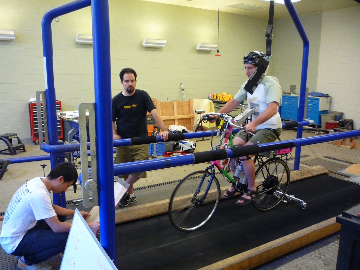
Sideview of the horse treadmill while Luke was riding the bicycle.
Pavilion
The bicycle was designed in such a way that all of the data collection equipment was on board and was suitable for data collection in a free environment. After lengthy bureaucratic negotiations, we were able to make use of the UCD pavilion floor for the experiments, Figure 11.2. The floor was made of a stiff rubber[3] and provided a rectangular, wind-free space of about 100’ by 180’ (30 m by 55 m). We rode around the perimeter to build up speed and did our maneuvers on a straight section about 100 feet (30 m) long. We were not able to travel at speeds higher than about 7 m/s as the tires would slip in the final turn into the test section (this seemed to be due to the dust on the floor). This indoor environment provided a wind free area which was more akin to the environment bicyclists normally ride in than did the treadmill.
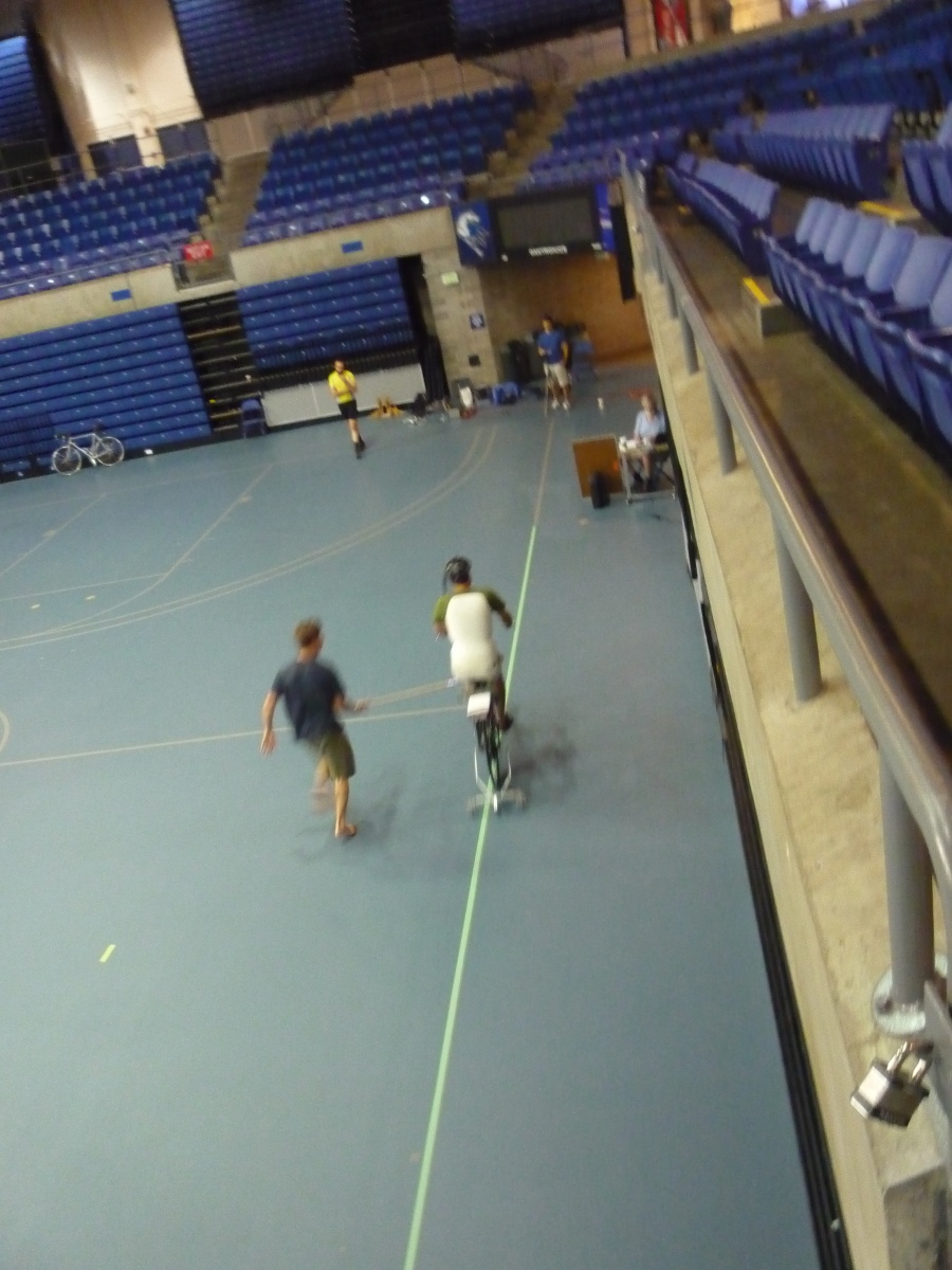
Overhead view of the pavilion floor during a perturbation run.
Maneuvers
Our choice of maneuvers was primarily guided by our previous experiments and the search for an optimal way to externally excite the system. We also made sure to perform sets of experiments that would act as a control without deliberate disturbances. The following list details the meaning of the maneuver labels in the dataset.
- System Test
- This is a generic label for data collected during various system tests that should not be used for general analysis. This was primarily used to check that all sensors were working before each set of experiments.
- Balance
- The rider is instructed to simply balance the bicycle and keep a relatively constant heading. They were instructed to focus on a point of their choosing in the far distance. There was an open door in front of the treadmill which allowed the rider to look to a point outside across the street. In the pavilion, the rider looked into the rafters of the building or at the furthest wall. We may have given slightly different instructions to the riders and Charlie did not understand the instructions exactly during some of the earlier runs, but nonetheless these can be analyzed with a control model that only has the roll and heading loops closed and maybe even with only the roll loop closed. We had a line taped to the pavilion floor during these runs that was still in the periphery of the rider’s vision. This may have affected their heading control even though they were instructed to ignore it.
- Balance With Disturbance
- Same as ‘Balance’ except that a lateral force perturbation is applied just under the seat of the bicycle. The rider wore a face shield on the side of the perturber so no visual cues were available to predict the perturbation time or direction. On the treadmill, we sample for 60 to 90 seconds with five to eleven perturbations per run. On the pavilion floor we were able to apply only two to four perturbations per run due to the length of the track. In the early runs (< 204), the lateral force was applied only in the negative direction (to the left) and the perturber decided when to apply the perturbations. For the later runs (> 203), we applied a random sequence of positive and negative perturbations that was unknown to the rider. On the treadmill, the rider signaled when they felt stable and the perturbation was applied at a random time between 0 and 1 second based on a simple computer program. On the pavilion floor, we simply applied the perturbations randomly but as soon as the rider felt stable so that we could get in as many as possible during each run.
- Track Straight Line
- The rider was instructed to focus on a straight line that was marked on the ground and he attempted to keep the front wheel on the line. The line of sight from the rider’s eyes to the line on the ground was essentially tangent the top of the front wheel. In the pavilion, the line could be seen up to 100 feet ahead, so there was greater peripheral view of the line. On the treadmill, there was from 0.5 to 1.5 meters of preview line available.
- Track Straight Line With Disturbance
- Same as “Track Straight Line” except that a lateral perturbation force is applied to the seat of the bicycle. This was done in the same fashion as described in “Balance With Disturbance”.
- Lane Change
- The rider attempted to track a line in similar fashion as the “Track Straight Line” maneuver except that the line was a single lane change. On the pavilion floor, the line was taped on the ground and the rider was instructed to do whatever felt best to stay on the line Figure 11.3. They could use full preview looking ahead, focus on the front wheel and line, or a combination of both. We also tried some lane changes on the treadmill but the lack of preview of the line made it especially difficult. We were able to manage it by marking a count down on the belt so that the rider new when the lane change would arrive. The rider also knew the direction of lane change beforehand for all the scenarios.
- Blind With Disturbance
- We did a run or two for each rider on the pavilion floor with the rider’s eyes closed to attempt to completely open the heading loop. In hindsight, blind tests would be preferable when identifying the rider control system so that only inner roll stabilization loop need be analyzed.
- Static Calibration
- We took a short duration sample of the sensors’ signals while no rider was on the bicycle and the bicycle was fixed as close as possible to vertical in roll before each set of runs. The static accelerometer readings could theoretically give the roll and pitch angles of the bicycle frame and be used to account for the bias in the roll angle measurements.
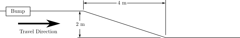
The dimensions of the single lane change on the pavilion floor for runs 115-139.
I only focus on the Balance and Track Straight Line maneuvers with and without disturbances in the following analyses and they will be referred to as Heading Tracking and Lateral Deviation Tracking in the text (as opposed to the labels in the database).
- Heading Tracking
- The rider was instructed to simply balance the bicycle and keep a relatively constant heading while focusing their vision at a point in the far distance.
- Lateral Deviation Tracking
- The rider was instructed to focus on a straight line that was marked on the ground and to attempt to keep the front wheel on the line.
Both tasks were performed with and without the application of a manually applied lateral perturbation force just below the seat. The forces were applied randomly in direction and time.
Data
The experimental data was collected on seven different days. The first few days were mostly trials to test the equipment, procedures and different maneuvers. The data from the trial days is valid data and we ended up using it in our analysis. The tires were pumped to 100 psi at the start of each day.
- February 4 2011 Runs 103-109
- These were the first trials on the treadmill for preliminary testing. Only Jason rode. We performed lateral deviation tracking with disturbances. The bike fell over, broke and we had to cut it short.
- February 28, 2011 Run 115-170
- These were the first trials in the pavilion. Jason was the only rider. We tried lane changes (115-139), lateral deviation tracking with disturbances (140-157), and a mixture of heading tracking and lateral deviation tracking with no disturbances (158-170). I noted that the slip clutch backlash seemed to be larger than the previous day with a guess of about 1 degree.
- March 9, 2011 Runs 180-204
- This was the second go at the treadmill, still just testing things. Jason was the only rider. We did heading and lateral deviation tracking with disturbances and some lane changes. The lane changes were 0.25 m wide left and right maneuvers back and forth among two lines on the treadmill at 2 m long segments. Countdown markers to give an idea when the lane change started were necessary due to the rider’s limited preview distance. We did the highest speed during any subsequent trials at 9 m/s. The 9 m/s runs generated a large amount of noise in the lateral force channel. The treadmill elevation was set at 0.1% upwards incline (because it was stuck).
- August 30, 2011 Runs 235-291
- Jason and Luke rode and performed heading and lateral deviation tasks with and without perturbations at three speeds on the treadmill.
- September 6, 2011 Runs 295-318
- Charlie performed heading and lateral deviation tasks with and without perturbations on the treadmill.
- September 9, 2011 Runs 325-536
- Luke, Charlie and Jason performed heading and lateral deviation tracking tasks on the Pavilion floor with and without perturbations. Most of Luke and Charlie’s runs were corrupt due to the time synchronization issues.
- September 21, 2011 Runs 538-706
- Luke and Charlie repeated the runs from September 9th. And we added a couple of blind runs for each of them.
The meta data and raw time history data for each run and all sensor calibration data were stored in individual Matlab mat files on the data acquisition computer using the BicycleDAQ software. The run files and calibration files are automatically numbered in sequence with a five digit number; one sequence for runs and one for calibrations. These mat files were then parsed and merged into a uniform, organized, and complete single HDF5 database that could be accessed by a number of programs and languages for fast data queries. I made use of PyTables for writing and reading from the database. The software BicycleDataProcessor was designed as an interface to the data in the database. In particular, it is able to load the raw data from individual runs, process it, and present it for easy manipulation and viewing.
The database is initially structured with three top-level tables and nodes containing the time histories of the sensors for each run. The run table has a row for each run and the columns store each piece of meta data, including the corruption coding described below. The signal table has a row for each raw and processed signal type and the classification information for each. The calibration table has a row for each calibration which provides information about the sensor and the data collected in the calibration.
We recorded a large set of meta data for each run to help with parsing during analyses. We also video recorded all of the runs (minus a few video mishaps). I coded each run based on the notes, data quality, and viewing the video for potential or definite corrupted data with the following five codes.
- Corrupt
- If the data is completely unusable due to time synchronization issues or others then this is set to true.
- Warning
- Runs with a warning flag are questionable and potentially not usable.
- Knee
- The rider’s knees would sometimes de-clip from the frame during a perturbation. This potentially invalidates the rigid rider assumption. An array of 15 boolean values, one for each perturbation in the run, are stored for each run and each true value in the array represents an individual perturbation where a knee disengaged with the bicycle.
- Handlebar
- On the treadmill the bicycle handlebars occasionally contacted the side railings. Each perturbation during the run in which this happened was recorded.
- Trailer
- On the treadmill the roll trailer occasionally contacted the side of the treadmill. Each perturbation during the run which this happened was recorded.
We ultimately collected 600+ runs that were potentially usable for analysis. Figure 11.4 gives a breakdown of the runs by rider, environment, maneuvers, and speed bins.
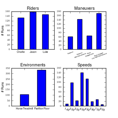
Four bar charts showing the number of runs that are potentially usable for model identification. These include runs from the treadmill and pavilion, one of the four primary maneuvers, and were not corrupt. Generated by src/systemidentification/data_histograms/py.
The processed data provides filtered signals that correspond to the coordinates and speeds outlined in our models, Chapters Bicycle Equations Of Motion and Extensions of the Whipple Model. We were even able to estimate the path of the wheel contact points on the ground. The quality of the data is high with little to no missing data and complete descriptions of the dynamic state through time. Figures 11.5 and 11.6 give examples of the processed data for the two environments.
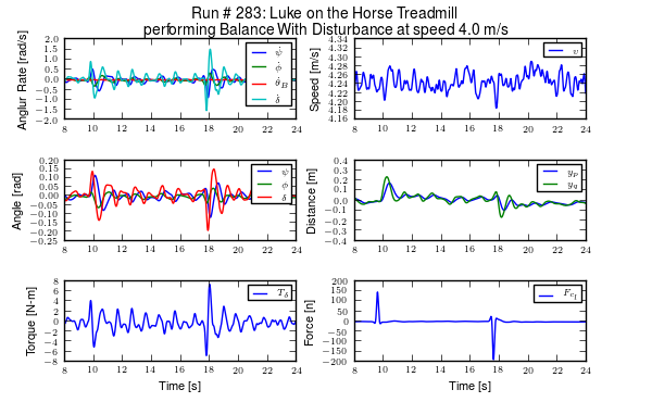
The time histories of the computed signals for a typical treadmill run after processing and filtering. Only a portion of the 90 second run is shown for clarity. Generated by src/systemidentification/run_time_history.py.
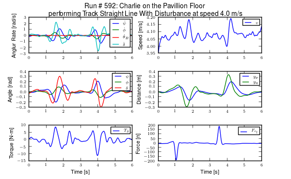
The time histories of the computed signals for a typical pavilion run after processing and filtering. Generated by src/systemidentification/run_time_history.py.
System Identification
My primary goal in the following analyses of all the collected data is to identify the manual control system employed the rider. I will approach this in a similar fashion to [Eat73b] and attempt to identify the plant, i.e. the open loop bicycle and rider dynamics, first followed by an identification of the control system. The question arises as to what the plant and controller consist of. In this case, I consider the plant to include the passive or open loop model of the bicycle combined with the rider’s biomechanics and the controller to be the some makeup of the human brain which takes sensory inputs, has time delays, and sends outputs for muscular control.
This two part process was not originally thought to be needed and I started with the identification of the control system assuming the Whipple model would be adequate for the open loop dynamics. But my preliminary attempts at identifying the controller with the Whipple model in place showed that the plant always under-predicted the steer torque needed for a given measured trajectory. This lead me into the exploration of the validity of the Whipple model.
There is actually very little experimental validation of the open loop dynamics of the bicycle, with [Koo06] being one of the better studies. But his study was limited to a riderless bicycle in a narrow speed range where the bicycle was stable. Taking the validity of first principles models like this for granted can potentially lead to inaccurate conclusions. In our case, it resulted in erroneous early estimations of the controller parameters. As pointed out by many, in particular the motorcycle researchers, there is very good reason to question some of assumptions. The main questionable assumption being knife-edge no side-slip wheels, especially when under a rider’s weight. And secondly, the rider’s biomechanics have much more influence and coupling to the bicycle than the motorcycle, which must be accounted for.
After a model for the open loop system is derived I identify parameters in the control structure described in [HMH12] and in Chapter Control. We’ve shown that this control structure is robust for a range of speeds and lends itself to the dictates of the crossover model which is built upon strong experimental evidence in human operator modeling. I make use of multi-input multi-output grey box state space identification techniques to arrive at the optimal parameters for the measured data.
Before I proceed, it is important to emphasize the difference in identifying a model that best predicts the data and identifying physical parameters in a model structure that cause the predictions to best fit the measured data. In the first case, it is somewhat easy to fit a model to input and output data. By increasing the order of the model and thus the number of free parameters one can theoretically fit every data point. This is most evident in the over-fitting of a linear trend with that of a higher order polynomial. It still often takes human intuition and reasoning to limit the order of the system to something that represents the true relationships between the variables. But even in this case, the individual meaning of the resulting identified parameters of a black box system may have little apparent connection to the known first principles laws we are familiar with and trust. In dynamics, we often want to know how well our first principles models predict the measured motion and secondly we’d like the ability to identify parameters, particularly ones we are uncertain of in the first principles models, from the measured data. Accurately identifying model parameters is much more difficult task, because noises, both process and measurement, have to be accounted for to get repeatable and accurate estimates of the parameters. I have had good success with finding models that predict the data but little success with explicit and accurate parameter identification in the following analyses. There is great room for improvement in the parameter identification if the noise issues are better managed.
Bicycle Model Validity
The open loop dynamics of the bicycle-rider system can be described using many models, see [ASKL05], [LS06], and [MPRS07] for good overviews. The benchmarked Whipple model [MPRS07] provides a somewhat minimalistic model in a manageable analytic framework which is capable of describing the essential dynamics such as speed dependent stability, steer and roll coupling, and non-minimum phase behavior. I use this model as the standard base model to work with, as the fidelity of simpler models are generally not adequate. The model is 4th order with roll angle, steer angle, roll rate and steer rate typically selected as the independent states and with roll and steer torque as inputs. I neglect the roll torque input and in its place extend the model to include a lateral force acting at a point on the frame to provide a new input, accurately modelling imposed lateral perturbations (see Chapter Extensions of the Whipple Model for the details). I also examine a second candidate model which adds inertial effects of the rider’s arms to the Whipple model, also in Chapter Extensions of the Whipple Model. This model was designed to more accurately account for the fact that the riders were free to move their arms with the front frame of the bicycle. This model is similar in fashion to the upright rider in [SK10a], but with slightly different joint definitions. Constraints are chosen so that no additional degrees of freedom are added, keeping the system both tractable and comparable to the benchmarked Whipple model.
I make the assumptions that the model is (1) linear and (2) has two degrees of freedom. The best model for a given set of data is constrained by those two assumptions. The implications of this is that even if the model predicts the outputs from the measured inputs it may not reflect realistic parameter values in a first principles sense because all real systems have infinite order. Secondly, the identified model may not map to the assumption we make in first principles derivations about things such as joints, friction, inertia, etc. There may exist higher order models which both fit the output data well and better map parameter values to first principle constructs. For example, a bicycle model with side slip at each wheel will be sixth order and if the regression to find the best model has extra degrees of freedom in the two additional equations, the optimal solution may be such that the numerical values of the equation coefficients map more closely to the first principle parameters. For example, it may be possible to make a fourth order model behave similarly to a sixth order model with “correct” first principles parameters by choosing unrealistic parameter values. But if the primary goal is the control identification, rather than understanding the quality of our first principles derivations, the model of lowest order that still fits the data well is completely suited for the task.
I estimated the physical parameters of the first principles models with the techniques described in Chapter Physical Parameters. The bicycle was measured to get accurate estimates of the parameters used in the benchmark bicycle. Each rider’s inertial properties were estimated using Yeadon’s [Yea90b] method which allowed easy extraction of body segment parameters for more complicated rider biomechanic models such as the inclusion of moving arms as described above. The parameter computation is handled with two custom open source software packages [Dem11] and [MKSH11].
State Space Realization
During all of the experiments there are two measured external (or exogenous) inputs: the steer torque and the lateral force. Both inputs are generated manually, the first from the rider and the second from the person applying the pulsive perturbation. The outputs can be any subset of the measured kinematical variables or combinations thereof. The problem can then be formulated as follows: given the inputs and outputs of the system and some system structure, what model parameters give the best prediction of the output given the measured input. This a classic system identification problem.
Method
For this analysis, I limit the inputs to steer torque and lateral force and the outputs to roll angle, steer angle, roll rate, and steer rate. The ideal fourth order system can be described with the following continuous state space description
where \(\eta(t)\) are the outputs and \(\mathbf{H}\) is the identity matrix.
Assuming that this model structure can adequately capture the dynamics of interest of the bicycle-rider system, our goal is to accurately identify the unknown parameters \(\theta\) which are made up of the unspecified entries in the \(\mathbf{F}\) and \(\mathbf{G}\) matrices. To do this one needs to recognize that this continuous formulation is not compatible with noisy discrete data. The following difference equation can be assumed if we sample the continuous system at \(t=kT\), \(k=1,2,\dots\), with \(T\) being the sample period and making the assumption that the variables are constant over the sample period (i.e. zero order hold).
The additional terms \(w\) and \(v\) represent the process and measurement noise vectors, respectively, which are assumed to be sequences of white Gaussian noise with zero mean and some covariance. By making use of the Kalman filter, Equation (2) can be transformed such that the optimal estimate of the states, \(\hat{x}\), with respect to the process and measurement noise covariance are utilized, see [Lju98].
where \(\mathbf{K}\) is the Kalman gain matrix. \(\mathbf{K}\) is a function of \(\mathbf{A}(\theta)\), \(\mathbf{C}(\theta)\) and the covariance and cross covariance of the process and measurement noises, but it can also be directly parameterized by \(\theta\). With that, this equation is called the directly parameterized innovations form [Lju98] and the entries of the four matrices in equation (3) can be estimated directly.
The \(\mathbf{A}\) and \(\mathbf{B}\) matrices are related to \(\mathbf{F}\) and \(\mathbf{G}\) by
where \(T\) is the sampling period. With a linear assumption \(\mathbf{A}\) and \(\mathbf{B}\) can even be directly estimated in discrete form by
The one step ahead predictor for the innovations form is
where \(q\) is the forward shift operator (\(q u(t) = u(t+1)\)) [Lju98]. The predictor is a vector of length \(p\) where each entry is a ratio of polynomials in \(q\). These are transfer functions in \(q\) from the previous inputs and outputs to the current output. In general, the coefficients of \(q\) are non-linear functions of the parameters \(\theta\).
We can now construct the cost function, which will enable the computation of the parameters which give the best fit using optimization methods. We’d like to minimize the error in the predicted output with respect to the measured output at each time step. First form \(Y_N\) which is a \(pN \times 1\) vector containing all of the current outputs at time \(kT\).
where \(p\) is the number of outputs and \(N\) is the number of samples. Then organize the predictor vector, \(\hat{Y}_N(\theta)\), the one step ahead prediction of \(Y_N\) given \(y(s)\) and \(u(s)\) where \(s \leq t - 1\)
The cost function is then the norm of the difference of \(Y_N\) and \(\hat{Y}_N(\theta)\) for all \(k\).
The value of \(\theta\) which minimizes the cost function is the best prediction
where \(Z^N\) is the set of all the measured inputs and outputs.
In general, the minimization problem is not trivial and may be susceptible to many of the issues associated with optimization including local minima. The number of unknown parameters in the \(\mathbf{K}\) matrix is a function of the number of states and the number of outputs, in our case in \(\mathbf{R}^{4\times4}\) which more than doubles the number of unknowns present in the \(\mathbf{A}\) and \(\mathbf{B}\) matrices. It is thus critical to reduce the number of unknown parameters to have a higher chance of finding the global minimum of the cost function. The accuracy of the system parameters depends on the ability to estimate the \(\mathbf{K}\) matrix along with the other parameters.
Before identification I further processed all of the signals that were generally symmetric about zero by subtracting the means over time. For some of the pavilion runs, this may have actually introduced a small bias, as the short duration runs with unbalanced perturbations may not have zero mean.
I made use of the Matlab System Identification Toolbox for the identification of the parameters \(\theta\) in each run of this model structure. In particular, a structured idss object was built with the initial guesses of the unknown parameters based on the Whipple model and the initial guesses for the initial conditions and the Kalman gain matrix being equal to zero. All of my attempts at identifying the Kalman gain matrix were plagued by local minima.
Results
It turns out that finding a model that meets the criterion is not too difficult when the output error form is considered (\(\mathbf{K}=0\)). This model may be able to explain the data well, but the parameter estimation is potentially poor because the parameters in the state and input matrices are adjusted such that the results fit both the true trajectories and the noise. Global minima in the search routine are quickly found when the number of parameters is between 10 and 14. When the \(\mathbf{K}\) matrix is added the number of unknown parameters increases by 16 and the global minimum becomes more difficult to find and I was rarely able, if ever, to find the global minimum for the general problem, even when reducing the number of outputs to one.
Figure 11.7 shows typical example input and output data for a single run (#596) with both steer torque and lateral force as inputs. The plot compares the simulation response of the input to the measured response. Notice that the identified model predicts the trajectory extremely well. Similar results are found for the majority of the runs. The Whipple model predicts the trajectory directions but the magnitudes are large, meaning that for a given trajectory, the Whipple model requires less torque than that measured. The Whipple model with the arm inertial effects does a better job than the basic Whipple model, but still has some magnitude differences with respect to the identified model. It also has a harder time predicting the roll angle than both the identified model and the Whipple model.
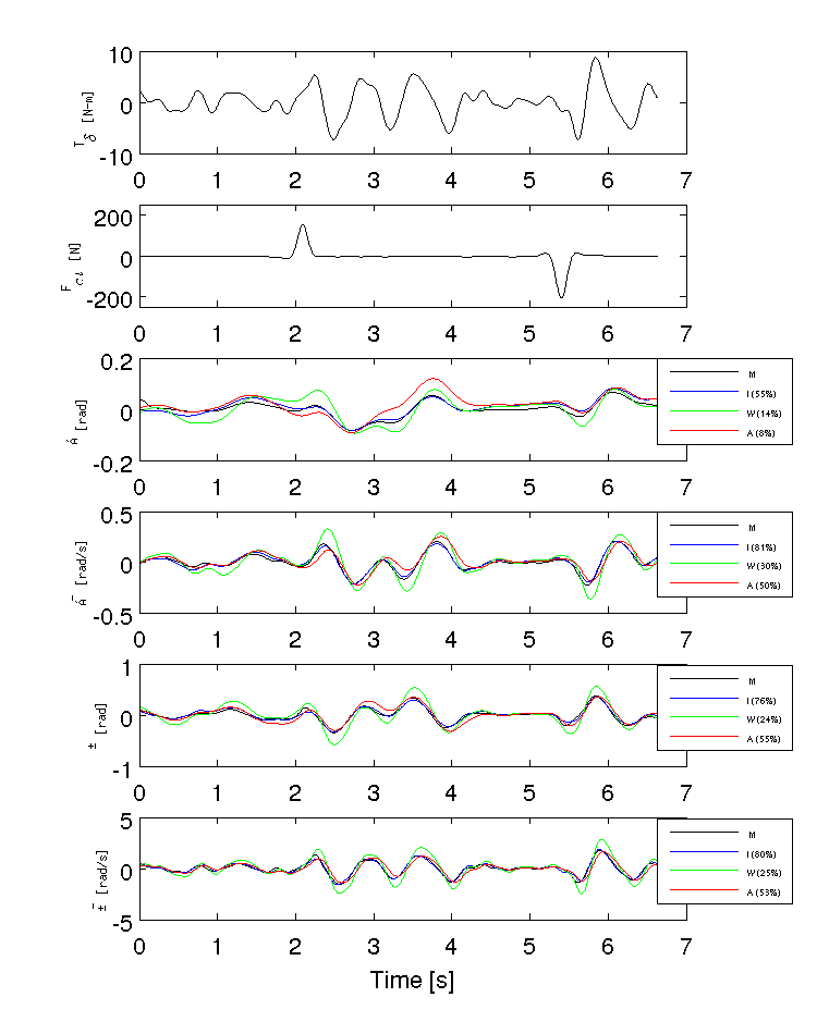
Example results for the identification of a single run (#596). The experimentally measured steer torque and lateral force are shown in the top two graphs. All of the signals were filtered with a 2nd order 15 hertz low pass Butterworth filter. The remaining four graphs show the simulation results for the Whipple model (W), Whipple model with the arm inertia (A), and the identified model for that run (I) plotted with the measured data (M). The percentages give the percent of variance explained by each model.
The identified models are almost always unstable due to the high weave critical speed and, even though the measured inputs stabilize the true system, they will not necessarily stabilize the models. This poses an issue when gauging the model quality by the percentage variance of the output data explained by the model. A model that blows up during the simulation may not necessarily be a bad model, but it will return a very small percent variance and lose its ability to be compared by that criterion. [BBCL03] and [TJ10] both are able to run feed-forward simulations of their motorcycle models with the measured steering torque. They both are dealing with high speed motorcycles which typically only have a slightly unstable capsize mode. [TJ10] uses a controller to compensate the torque for unbounded errors so that the simulation doesn’t blow up. The method I use here is to choose short duration portions of the runs for simulation and search for the best set of initial conditions to keep the model stable during the duration. This generally works but there are ultimately some incomparable runs due to this issue.
I use this structured state space output error identification procedure for a collection of experiments (\(n=368\)) over a range of speeds between about 1 and 9 m/s. Figures 11.8 and 11.9 plot the identified coefficients of the dynamical equations of motion (i.e. the bottom two rows of the \(\mathbf{F}\) and \(\mathbf{G}\) matrices) as a function of speed for all of the experiments using box plots. Both the Whipple (green) and arm (red) model predictions are superimposed for comparison. The first notable thing is that the coefficients seem to generally have large variance, especially as the speed increases. Secondly, the roll acceleration, \(\ddot{\phi}\), equation seems to be better predicted by the two models and the data has less spread at the lower speeds, barring the \(\dot{\phi}\) coefficient which has large spread and no apparent relationship with speed for both equations. The roll equation also seems to have less spread in the experimental data. For example, the \(a_{\ddot{\phi}\delta}\) coefficient appears to be very tight and the first principles models predict it very well. The constant, linear, and quadratic trends in the coefficients are somewhat visible in the data but the variance in the coefficients clouds it. This variability in the coefficient predictions depends on many things including data quality, the ability to identify a process noise model, speed being constant during the run, choice of unknown coefficients, and more. With all of these improved, detailed regression models may be able to reveal the true trends[4]. Nonetheless, these graphs reveal several important things:
- The identified models predict the data well with most having mean predicted variance of the four outputs above 70% (but this is tightly coupled to run duration, i.e. longer runs have more room for model error).
- Some of the coefficients are well predicted by the Whipple model and can be fixed from first principles calculations, notably: \(a_{\ddot{\phi}\phi}\), \(a_{\ddot{\phi}\delta}\) and \(b_{\ddot{\delta}T_\delta}\) and maybe even \(a_{\ddot{\delta}\delta}\).
- The roll rate coefficients are highly variable with poor prediction by the models. Deficiencies in the first principles models are likely.
- Either the higher speed runs are outliers, or the behavior of the system changes more rapidly with speeds above 5 m/s or so.
- Some coefficients spread around zero giving inconsistent signs and others give opposite signs from those the first principles models expect.
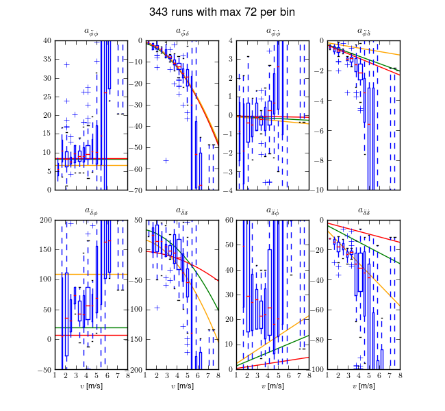
State coefficients of the linear dynamical equations of motion plotted as a function of speed. Each box plot represents the distribution of that parameter for a small range of speeds, i.e. speed bin. The width of the box is proportional to the total duration of the runs in that speed bin. The green line is the Whipple model and the red line is the arm model. Only experiments with a mean fit percentage greater than zero are shown. The orange line is the model identified with the canonical method using runs done by Luke in the pavilion which is presented and discussed in the next section. Generated by src/systemidentification/coefficient_box_plot.py.
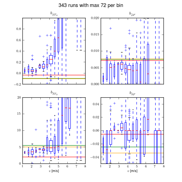
Input coefficients of the linear dynamical equations of motion plotted as a function of speed. Each box plot represents the distribution of that parameter for a small range of speeds, i.e. speed bin. The width of the box is proportional to the total duration of the runs in that speed bin. The green line is the Whipple model and the red line is the arm model. Only experiments with a mean fit percentage greater than zero are shown. The orange line is the model identified with the canonical method using runs done by Luke in the pavilion which is presented and discussed in the next section. Generated by src/systemidentification/coefficient_box_plot.py.
Figure 11.10 gives another view of the resulting data. It is a frequency response plot at the mean speed for a set of runs. The blue lines give the mean and one standard deviation bounds of the magnitude and phase of the system transfer function \(\frac{\phi}{T_\delta}(s)\) for the set of runs. Even though the spread in the identified parameters seems high in Figures 11.8 and 11.9, the Bode plot shows that the identified system frequency response is not as variable, especially in magnitude. It is also apparent that the experimental magnitude mean has a -5 to -10 dB offset across the frequency range shown with respect to the Whipple model, although the Whipple model does fall within one standard deviation of the mean. This correlates with the amplitude differences in the trajectories shown in Figure 11.7. Notice that the arm model has little to no offset between 2 and 10 rad/s, thus the better amplitude matching. The frequency response may give a better indication of the overall identified model quality.
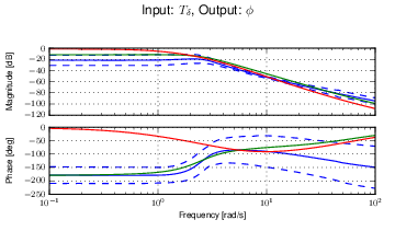
Frequency response of steer torque to roll angle for a set of runs at \(4.0 \pm 0.3\) m/s. The solid blue line is the mean from the identified runs and is bounded by the standard deviation, the dotted blue lines. The green line is the Whipple model and the red line is for the model which accounted for the arm inertial effects.
Conclusion
I have shown that a fourth order structured state space model is both adequate for describing the motion of the bicycle under manual control in a speed range from approximately 1.5 m/s to 9 m/s. The fact that higher order models may not be necessary for bicycle dynamic description is an important finding. More robust models of single track vehicles are typically higher than 4th order, with degrees of freedom associated with tire slip, frame flexibilities, and rider biomechanics. These findings suggest that the more complex models may be overkill for many modeling purposes. The data subsequently also reveals that fourth order archetypal first principles models are not robust enough to fully describe the dynamics. The deficiencies are most likely due to un-modeled effects, with the knife-edge, no side-slip wheel contact assumptions being the most probable candidate. Un-modeled rider biomechanics such as passive arm stiffness and damping and head motion may play a role too. The uncertainty in the estimates of the physical parameters from Chapter Physical Parameters is not large enough to explain the difference between the identified coefficient identification and their predictions from first principles. It is likely that something as simple as a “static” tire scrub torque is needed to improve the fidelity of the first principles derivations, but that doesn’t preclude that the additional of a tire slip model might also improve the models.
Canonical Identification
One issue I faced with the state space realization was dealing with multiple experiments. Ideally I had hoped to identify a linear model that was a function of speed with respect to all or various subsets of the experiments. It is possible to concatenate runs, but discontinuities in the data potentially disrupt the identification. There is also the possibility of designing a cost function that gives the error in all the outputs across all of the runs simultaneously instead of on a per run basis. Both my recently obtained knowledge in system identification and the constraints of the methods available in the Matlab System Identification toolbox were limiting factors in these two approaches. But, Karl Åström suggested doing the system identification with respect to the second order form of the equations of motion. This would allow one to use both simple least squares for the solution and the ability to compute models from large sets of runs. This section deals with this approach.
Model structure
The identification of the linear dynamics of the bicycle can be formulated with respect to the benchmark canonical form realized in [MPRS07], Equation (11). If the time varying quantities in the equations are all known at each time step, the coefficients of the linear equations can be estimated given enough time steps.
where the time-varying states roll and steer are collected in the vector \(q = [\phi \quad \delta]^T\) and the time varying inputs roll torque and steer torque are collected in the vector \(T = [T_\phi \quad T_\delta]^T\). This equation assumes that the velocity is constant with respect to time as the model was linearized about a constant velocity equilibrium, but the velocity can also potentially be treated as a time varying parameter if the acceleration is negligible. I extend the equations to properly account for the lateral perturbation force, \(F\), which was the actual input we delivered during the experiments. It contributes to both the roll torque and steer torque equations.
where \(H = [H_{\phi F} \quad H_{\delta F}]^T\) is a vector describing the linear contribution of the lateral force to the roll and steer torque equations. \(H_{\phi F}\) is approximately the distance from the ground to the force application point. \(H_{\delta F}\) is a distance that is a function of the bicycle geometry (trail, wheelbase) and the longitudinal location of the force application point. For our normal geometry bicycles, including the one used in the experiments, \(H_{\delta F} << H_{\phi F}\). I estimate \(H\) for each rider/bicycle from geometrical measurements and the state space form of the linear equations of motion calculated in Chapter Extensions of the Whipple Model.
where \(x = [\phi \quad \delta \quad \dot{\phi} \quad \dot{\delta}]^T\) and \(u = [F \quad T_\phi \quad T_\delta]^T\). The state and input matrices can be partitioned.
where \(\mathbf{A}_l\) and \(\mathbf{A}_r\) are the 2 x 2 sub-matrices corresponding to the states and their derivatives, respectively. \(\mathbf{B}_F\) and \(\mathbf{B}_T\) are the 2 x 1 and 2 x 2 sub-matrices corresponding to the lateral force and the torques, respectively. The benchmark canonical form can now be written as
where
| Rider | \(H\) |
| Charlie | \([0.902 \quad 0.011]^T\) m |
| Jason | \([0.943 \quad 0.011]^T\) m |
| Luke | \([0.902 \quad 0.011]^T\) m |
The location of the lateral force application point is the same for Charlie and Luke because they used the same seat height. The force was applied just below the seat, which was adjustable in height for different riders.
Data processing
Chapter Davis Instrumented Bicycle details how each of the signals were measured and processed. For the following analysis, all of the signals were filtered with a second order low pass Butterworth filter at 15 Hz. The roll and steer accelerations were computed by numerically differentiating the roll and steer rate signals with a central differencing method except for the end points being handled by forward and backward differencing. The mean was subtracted from all the signals except the lateral force.
Identification
A simple analytic identification problem can be formulated from the canonical form. If we have good measurements of \(q\), their first and second derivatives, forward speed \(v\), and the inputs \(T_\delta\) and \(F\), the entries in \(\mathbf{M}\), \(\mathbf{C}_1\), \(\mathbf{K}_0\), \(\mathbf{K}_2\), and \(H\) can be identified by forming two simple regressions, i.e. one for each equation in the canonical form. I use the instantaneous speed at each time step rather than the mean over a run to improve accuracy with respect to the speed parameter as it has some variability.
The roll and steer equation each can be put into a simple linear form
where \(\Theta\) is a vector of the unknown coefficients and \(\mathbf{\Gamma}\) and \(Y\) are made up of the inputs and outputs measured during a run. \(\Theta\) can be all or a subset of the entries in the canonical matrices. If there are \(N\) samples in a run and we desire to find \(M\) entries in the equation, then \(\mathbf{\Gamma}\) is an \(N \times M\) matrix and \(Y\) is an \(N \times 1\) vector. The Moore-Penrose pseudo inverse can be employed to solve for \(\Theta\) analytically. The estimate of the unknown parameters is then
For example, if we fix the mass terms in the steer torque equation and let the rest be free the linear equation is
The error in the fit is
The covariance of \(\Theta\), Equation (23), of the parameter estimations can be computed with respect to the error.
Equations (19), (21), (22), and (23) can be solved for each run individually, a portion of a run, or a set of runs. Secondly, all of the parameters in the canonical matrices need not be estimated. The analytical benchmark bicycle model [MPRS07] gives a good idea of which entries in the matrices we may be more certain about from our physical parameters measurements in Chapter Physical Parameters. I went through the benchmark formulation and fixed the parameters based on these rules, keeping in mind that even little numbers can have large effects to the resulting dynamics:
- If the parameter is greatly affected by trail, leave it free.
- If the parameter is greatly affected by the front assembly moments and products of inertia, leave it free.
- If the parameter is identically equal to zero, fix it.
The reasoning for these assumptions are:
- Trail is difficult to measure and be certain about, especially since the bicycle tire deforms and creates a variable shaped tire contact patch which depends on the tires properties, pressure, and the configuration of the bicycle. The true trail is what is typically called pneumatic trail and gives the location in the tire patch at which the resultant contact force acts.
- The front frame moments and products of inertia play a large role in the steer dynamics and I’m not as confident in the estimation of these due to the fact that our apparatus was more suited to the estimate the inertial properties of the rear frame than the front.
- The zero entries in the velocity dependent stiffness and damping matrices that correspond to the roll angle and rate are assumed to hold from first principles.
For the roll equation this leaves \(M_{\phi\delta}\), \(C_{1\phi\delta}\), and \(K_{0\phi\delta}\) as free parameters, and for the steer equation this leaves \(M_{\delta\phi}\), \(M_{\delta\delta}\), \(C_{1\delta\phi}\), \(C_{1\delta\delta}\), \(K_{0\delta\phi}\), \(K_{0\delta\delta}\), \(K_{2\delta\delta}\), and \(H_{\delta F}\) as free parameters.
I start by identifying the three coefficients of the roll equation for the given data. This choice is due to there being more certainty in the roll equation estimates from first principles because there are fewer unknown parameters.
I then enforce the assumptions that \(M_{\phi\delta} = M_{\delta\phi}\) and \(K_{0\phi\delta} = K_{0\delta\phi}\) to fix these values in the steer equation to the ones identified in the roll equation, leaving fewer free parameters in the steer equation[5]. This symmetry is enforced to coincide with the theory and choice of coordinates. Finally, I identify the remaining steer equation coefficients with
Results
I selected data for three riders on the same bicycle, performing two maneuvers, in two different environments. There is little reason to believe the dynamics of the passive system should vary much with respect to different maneuvers, but there is potentially variation across riders due to the differences in their inertial properties and there may be variation across environments because of the differences in the wheel to floor interaction. I opted to compute the best fit model across series of runs to benefit from the large dataset. This leaves these four scenarios:
- All riders in both environments, one data set
- All riders in each environment, two data sets
- Each rider in both environments, three data sets
- Each rider in each environment, six data sets
| Rider | Environment | Number of runs | Number of time samples, \(N\) |
| (C)harlie | (H)orse treadmill | 24 | 267773 |
| (C)harlie | (P)avilion | 87 | 118700 |
| (C)harlie | (A)ll | 111 | 386473 |
| (J)ason | (H)orse treadmill | 57 | 804995 |
| (J)ason | (P)avilion | 93 | 112582 |
| (J)ason | (A)ll | 150 | 917577 |
| (L)uke | (H)orse treadmill | 25 | 272719 |
| (L)uke | (P)avilion | 88 | 125878 |
| (L)uke | (A)ll | 113 | 398597 |
| (A)ll | (H)orse treadmill | 106 | 1345487 |
| (A)ll | (P)avilion | 268 | 357160 |
| (A)ll | (A)ll | 374 | 1702647 |
A total of 12 different models can be derived from this perspective.
All riders in both environments
This section details the example results for one subset of data. Here I make the assumption that the best fit model doesn’t vary much across riders or environments. The assumption that the passive model of the bicycle and rider are similar with respect to rider can be justified by recognizing that the Whipple model predicts little difference in the dynamics with respect to the three bicycle/rider combinations. On the other hand, I have little reason to believe the environments are the same except that both floors are made of a rubber like material. I calculated the best fit over 374 runs giving about 142 minutes of data sampled at 200 Hz, \(N=1720647\).
The eigenvalues as a function of speed of the identified model can be compared to those of the Whipple and arm models, see Section Rider Arms in Chapter Extensions of the Whipple Model. Figure 11.11 shows the root locus of the three models. The oscillatory weave mode exists in all three models, with it always being stable in the arm model but being unstable at lower speeds in the other two models. The identified model’s oscillatory weave mode is unstable over most of the shown speed range. Above 3 m/s or so, the Whipple model’s oscillatory weave mode diverges from the identified model to different asymptotes. The arm model weave mode diverges somewhere in between. Note that the arm model has an unstable real mode for all speeds. Figure 11.12 gives a different view of the root locus allowing one to more easily compare the real parts of the eigenvalues. The imaginary parts of the weave mode have similar curvature with respect to speed for all the models, with the identified model having about 1 rad/s larger frequency of oscillation for all speeds. The identified model does have a stable speed range where the Whipple model under predicts the weave critical speed by almost 2 m/s. The identified caster mode is much faster than the one predicted by the Whipple model which is somewhat counterintuitive because tire scrub torques would probably tend to slow the caster mode. Although, the pneumatic trail and the rider’s arm inertia could play a larger role that expected. Furthermore, the caster mode may not be well identified because the experiments were not design to specifically excite it.
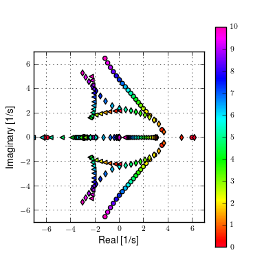
Root locus of the identified model (circle), the Whipple model (diamond), and the arm model (triangle) with respect to speed in m/s. Generated by src/systemidentification/canonical_plots.py.
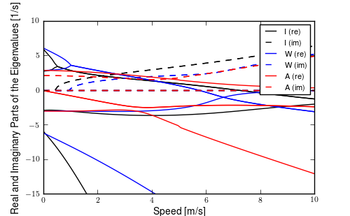
Real and imaginary parts of the eigenvalues as a function of speed for model (I)dentified from all runs, the (W)hipple model and the (A)rm model. Generated by src/systemidentification/canonical_plots.py.
The identification process is based on identifying the input/output relationships among measured variables. The frequency response provides a view into these relationships. Figures 11.13 to 11.16 give a picture of how the first principles models compare to the identified model with respect to frequency response from a roll torque input. The frequency band from 1 rad/s to 12 rad/s is of most concern as it bounds a reasonable range that the human may be able to operate within.
The roll torque to roll angle response Figure 11.13 shows that at 2 m/s (solid lines) the response of the Whipple model and the identified model are practically identical across the frequency range shown. On the other hand, the arm model predicts the high frequency (> 4 rad/s) behavior really well, but the magnitude is as great as 50 dB larger and the phase off by 180 degrees at lower frequencies. At 4 m/s the Whipple model still predicts the phase well, but the magnitudes do not match below 100 rad/s with 10 dB difference at lower frequencies. At this speed the arm model matches the identified model as low as 3.5 rad/s but the low frequency phase still being 180 degrees off. The magnitude of the identified model stays quite constant among the 4, 6, and 9 m/s models. As the speed increases the Whipple and arm models are less predictive of the identified model at low frequencies, but tend to match out past 4 rad/s or so.
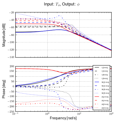
\(\frac{\phi}{T_\phi}\) frequency response of the three models, (I)dentified, (W)hipple, and (A)rm, at four speeds (2, 4, 6, and 9 m/s). The color indicates the model and the line type indicates the speed. Generated by src/systemidentification/canonical_plots.py.
Figure 11.14 shows the steer angle response with respect to the roll torque. Once again the Whipple model is almost identical to the identified model at the lowest speed, 2 m/s. The arm model has about a +5 dB offset at low frequencies and a -10 dB offset at high frequencies with the models only being similar just around 4 rad/s. At 9 m/s the Whipple model has similar magnitude and phase above 7 rad/s whereas the low frequency shows that the Whipple model has up to +30 dB magnitude difference with respect to the identified model. The arm model behaves in much the same way at 9 m/s.
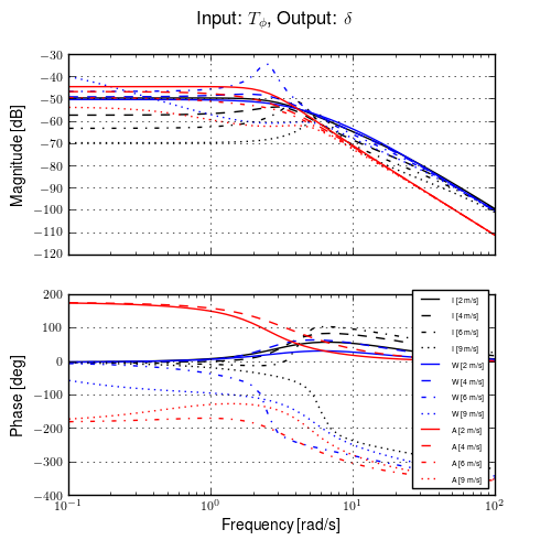
\(\frac{\delta}{T_\phi}\) frequency response of the three models, (I)dentified, (W)hipple, and (A)rm, at four speeds (2, 4, 6, and 9 m/s). The color indicates the model and the line type indicates the speed. Generated by src/systemidentification/canonical_plots.py.
The steer torque to roll angle transfer function, Figure 11.15 may be the most important to model accurately as it is the primary method of controlling the bicycle’s direction, i.e. commanding roll allows one to command yaw. At 2 m/s the Whipple model magnitude matches at lower frequencies (< 4 rad/s) better and the arm model better at higher frequencies (> 4 rad/s). A 4 m/s and above the magnitude of identified varies little with speed, which contrasts the stronger speed dependence of the first principles models. The low frequency behavior of the identified model is not well predicted by the Whipple and arm models at the three highest speeds but about about 3 rad/s the arm model shows better magnitude matches than the Whipple model.
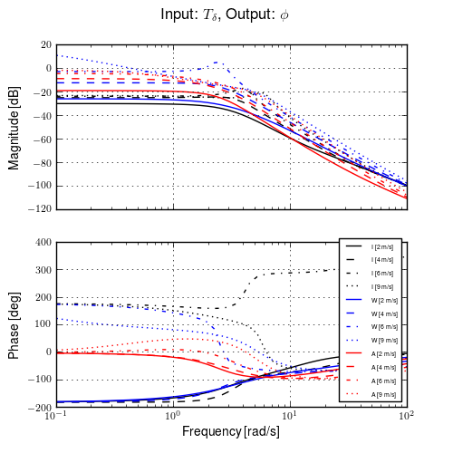
Frequency response of the three models, (I)dentified, (W)hipple, and (A)rm, at four speeds (2, 4, 6, and 9 m/s). The color indicates the model and the line type indicates the speed. Generated by src/systemidentification/canonical_plots.py.
The steer torque to steer angle frequency response, Figure 11.16, shows that at speeds above 2 m/s the first principle models do not predict the response well at low frequencies. The response changes more drastically with respect to speed for the first principles models than for the identified model.
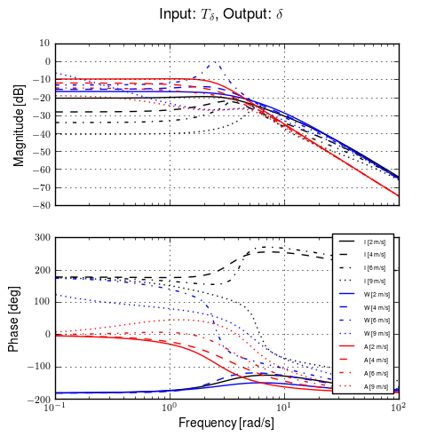
Frequency response of the three models at four speeds. The color indicates the model and the line type indicates the speed. Generated by src/systemidentification/canonical_plots.py.
Comparison of identified models
Tables 11.3, 11.4, and 11.5 present the identified canonical coefficient values from all twelve of the chosen data subsets. The variances of the coefficient estimates with respect to how well the model fits the data in the steer equation are quite low except for the \(H_{\delta F}\) parameter. The low variance is partially due to the large datasets but also due to the quality of the resulting fits. The \(H_{\delta F}\) is highly dependent on the trail which is expected to be difficult to identify. The coefficient estimates are not all repeatable among the data subsets. In particular \(C_{1\delta\phi}\) and \(H_{\delta F}\) have the largest relative variance among the models (> 62%). \(M_{\delta\delta}\), \(C_{1\phi\delta}\), \(C_{1\delta\delta}\), and \(K_{2\delta\delta}\) are the most consistent among the models (< 18%) with the remaining coefficients falling somewhere in between. This is odd because these data sets are not independent of one another where some are subsets of the others but once again the identification procedure does not explicitly account for process noise and the coefficient estimates reflect this. A sensitivity study for each coefficient with respect to the various physical parameters could help reveal which parameters less likely fit into the Whipple model mold.
| \(M_{\phi\delta}\) | \(C_{1\phi\delta}\) | \(K_{0\phi\delta}\) | ||||||||
|---|---|---|---|---|---|---|---|---|---|---|
| R | E | Value | \(\sigma\) | % Diff | Value | \(\sigma\) | % Diff | Value | \(\sigma\) | % Diff |
| A | H | 1.659 | 0.010 | -27.6% | 21.35 | 0.02 | -49.3% | -5.29 | 0.06 | 123.2% |
| C | H | 3.36 | 0.02 | 54.4% | 20.05 | 0.04 | -49.8% | -0.1 | 0.1 | -96.5% |
| L | P | 2.56 | 0.03 | 13.2% | 33.53 | 0.05 | -19.5% | -4.53 | 0.10 | 91.7% |
| J | P | 2.53 | 0.02 | 3.7% | 30.04 | 0.05 | -32.7% | -1.82 | 0.10 | -26.7% |
| C | A | 3.75 | 0.02 | 72.6% | 21.19 | 0.05 | -47.0% | -1.9 | 0.1 | -16.5% |
| L | H | 1.82 | 0.02 | -19.5% | 19.18 | 0.04 | -53.9% | -6.84 | 0.10 | 189.8% |
| A | A | 2.284 | 0.008 | -0.3% | 23.94 | 0.02 | -43.1% | -3.92 | 0.04 | 65.4% |
| J | H | 0.95 | 0.01 | -61.0% | 22.21 | 0.02 | -50.3% | -7.13 | 0.08 | 187.5% |
| L | A | 2.19 | 0.02 | -3.1% | 25.94 | 0.03 | -37.7% | -5.37 | 0.07 | 127.4% |
| A | P | 3.02 | 0.02 | 31.7% | 28.64 | 0.04 | -31.9% | -2.93 | 0.08 | 23.8% |
| J | A | 1.70 | 0.01 | -30.4% | 24.26 | 0.02 | -45.7% | -3.97 | 0.06 | 60.2% |
| C | P | 4.15 | 0.05 | 90.8% | 22.3 | 0.1 | -44.1% | -3.4 | 0.3 | 48.6% |
| \(M_{\delta\delta}\) | \(C_{1\delta\phi}\) | \(C_{1\delta\delta}\) | ||||||||
|---|---|---|---|---|---|---|---|---|---|---|
| R | E | Value | \(\sigma\) | % Diff | Value | \(\sigma\) | % Diff | Value | \(\sigma\) | % Diff |
| A | H | 0.2088 | 0.0003 | -5.3% | -0.891 | 0.002 | 183.0% | 1.5982 | 0.0008 | 14.8% |
| C | H | 0.1435 | 0.0007 | -34.0% | -0.881 | 0.006 | 179.6% | 1.601 | 0.002 | 19.5% |
| L | P | 0.2505 | 0.0009 | 14.2% | -0.549 | 0.009 | 74.2% | 2.100 | 0.003 | 52.6% |
| J | P | 0.1786 | 0.0007 | -20.4% | -1.09 | 0.01 | 246.6% | 1.915 | 0.002 | 31.0% |
| C | A | 0.1760 | 0.0008 | -19.1% | -0.380 | 0.008 | 20.7% | 1.675 | 0.002 | 25.0% |
| L | H | 0.2336 | 0.0007 | 6.5% | -1.058 | 0.005 | 235.8% | 1.726 | 0.002 | 25.5% |
| A | A | 0.2000 | 0.0003 | -9.2% | -0.888 | 0.002 | 182.0% | 1.7337 | 0.0008 | 24.5% |
| J | H | 0.2500 | 0.0005 | 11.5% | -0.849 | 0.003 | 169.6% | 1.545 | 0.001 | 5.7% |
| L | A | 0.2385 | 0.0006 | 8.7% | -1.053 | 0.004 | 234.4% | 1.943 | 0.002 | 41.3% |
| A | P | 0.1949 | 0.0006 | -11.6% | -0.236 | 0.007 | -24.9% | 1.872 | 0.002 | 34.4% |
| J | A | 0.2012 | 0.0003 | -10.2% | -0.953 | 0.002 | 202.4% | 1.6592 | 0.0009 | 13.5% |
| C | P | 0.220 | 0.002 | 1.3% | 0.84 | 0.02 | -366.5% | 1.702 | 0.005 | 27.0% |
| \(K_{0\delta\delta}\) | \(K_{2\delta\delta}\) | \(H_{\delta F}\) | ||||||||
|---|---|---|---|---|---|---|---|---|---|---|
| R | E | Value | \(\sigma\) | % Diff | Value | \(\sigma\) | % Diff | Value | \(\sigma\) | % Diff |
| A | H | -0.6055 | 0.0003 | -18.1% | 2.182 | 0.002 | -0.7% | 0.0064 | 0.0008 | -41.5% |
| C | H | -1.2406 | 0.0007 | 75.5% | 2.563 | 0.006 | 21.9% | 0.020 | 0.002 | 77.1% |
| L | P | -0.4889 | 0.0009 | -33.7% | 2.603 | 0.009 | 18.9% | 0.011 | 0.003 | -1.3% |
| J | P | -0.6561 | 0.0007 | -15.3% | 1.99 | 0.01 | -13.2% | 0.007 | 0.002 | -30.2% |
| C | A | -0.9017 | 0.0008 | 27.6% | 2.763 | 0.008 | 31.4% | 0.018 | 0.002 | 59.1% |
| L | H | -0.3181 | 0.0007 | -56.8% | 2.508 | 0.005 | 14.5% | 0.006 | 0.002 | -44.1% |
| A | A | -0.6678 | 0.0003 | -9.7% | 2.340 | 0.002 | 6.5% | 0.0086 | 0.0008 | -21.8% |
| J | H | -0.3579 | 0.0005 | -53.8% | 1.968 | 0.003 | -14.3% | -0.000 | 0.001 | -100.9% |
| L | A | -0.4614 | 0.0006 | -37.4% | 2.524 | 0.004 | 15.2% | 0.008 | 0.002 | -31.0% |
| A | P | -0.6003 | 0.0006 | -18.8% | 2.469 | 0.007 | 12.4% | 0.013 | 0.002 | 17.7% |
| J | A | -0.6207 | 0.0003 | -19.8% | 1.996 | 0.002 | -13.1% | 0.0047 | 0.0009 | -55.7% |
| C | P | -0.288 | 0.002 | -59.3% | 2.81 | 0.02 | 33.8% | 0.020 | 0.005 | 79.9% |
It is interesting to note that \(C_{1 \delta \phi}\) deviates quite significantly from the Whipple model prediction. This term depends on the wheel radii, wheel rotational inertia, wheelbase, steer axis tilt, and trail. All of these but trail are easily measured so it is tempting to solve for trail given \(C_{1 \delta \phi}\) and the other measured parameters described in [MPRS07].
The results for each data subset are given in Table 11.6. On average the values are extremely unrealistic when compared to the measured geometric trail of \(c=0.0599\) meters. This may imply that including the effects of pneumatic trail would not be enough to improve the predictive capabilities of the Whipple model. It also points to the potentially erroneous assumptions made in this identification effort such as the order of the system and which parameters are fixed. Even thought the model is quite adequate for describing the measured motion, it lacks the complexness to identify the precise deficients in the first principles assumptions.
| R-E | A-H | C-H | L-P | J-P | C-A | L-H | A-A | J-H | L-A | A-P | J-A | C-P |
|---|---|---|---|---|---|---|---|---|---|---|---|---|
| \(c\) [m] | 1.006 | 0.989 | 0.443 | 1.335 | 0.167 | 1.279 | 1.001 | 0.937 | 1.272 | -0.069 | 1.107 | -1.835 |
The measurement errors, model structure and order dictate how well the models can predict the input-output behavior of each run or even each perturbation. The ideal goal is to select one or a small set of models that do a good job at predicting the measured behavior for each run. The previous section’s state space methods have already shown that the Whipple and arm models may not provide adequate predictions.
Figures 11.17, 11.18, and 11.19 plot the steer torque to roll angle frequency response for three speeds: 2 m/s, 5.5 m/s and 9.0 m/s for each of the models in Tables 11.3, 11.4, and 11.5. At the lowest speed, all of the models have a similar frequency response, especially in the frequency band between about 1 an 20 rad/s. At 5.5 m/s the models are similar at a higher bandwidth, 4 to 30 rad/s, and at 9.0 m/s even higher, 10 to 50 rad/s. Notice that the frequency band where the models are most similar shifts to higher frequencies at higher speeds. The model derived from all of the data (all rider and all runs), gives an average model and if this model is significantly better at predicting the measured behavior of the Whipple and arm models, it may be a good general candidate model for this bicycle.
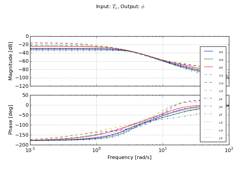
Steer torque to roll angle frequency responses at 2.0 m/s for all the identified models in Tables 11.3, 11.4, and 11.5.
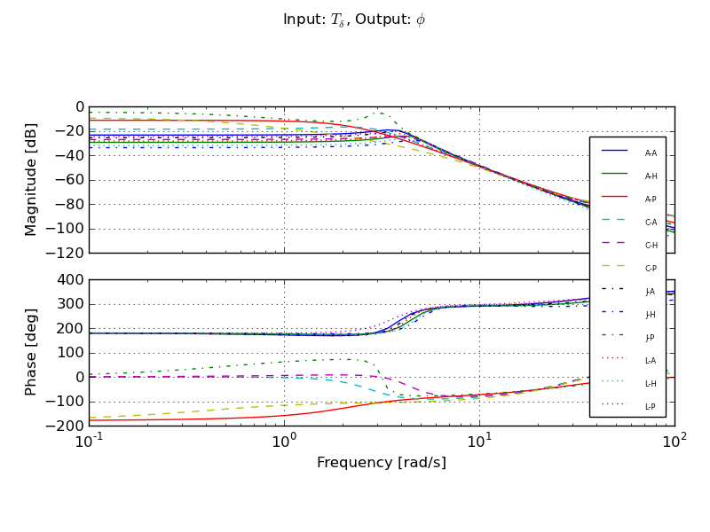
Steer torque to roll angle frequency responses at 5.5 m/s for all the identified models in Tables 11.3, 11.4, and 11.5.
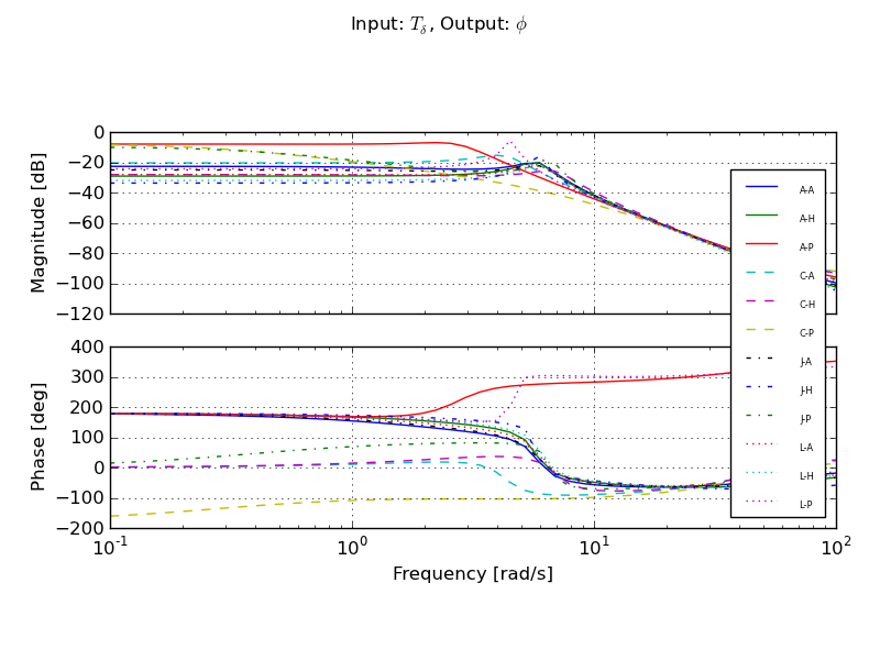
Steer torque to roll angle frequency responses at 9.0 m/s for all the identified models in Tables 11.3, 11.4, and 11.5.
The predictive capability and quality of a given model can be quantified by an assortment of criterion and methods. I’ve made use of two criterion to judge the quality of these models with respect to given data. The first is to simulate the system given the measured inputs. This method works well when the open loop system is stable, but if it is unstable as so in the case of this bicycle, it may be difficult to simulate. Searching for initial conditions that give rise to a stable model for the duration of the run or simulating by weighting the future error less may relieve the instability issues. Another option is to see how well the inputs are predicted given the measured outputs. The canonical form of the equations lend themselves to this and only two inputs per run need be checked.
The predicted torques on the system are
and the measured torques as
\(y_p\) and \(y_m\) can be computed for each run along with the variance accounted for (VAF), by the model for both the total roll torque and the steer torque
I compute the VAF for each of the 374 runs used in the canonical identification outlined in Equation (29) using each of the 12 identified models and both the Whipple and Arm models. This percentage can be used as a criterion with which to judge the ability of one model versus another to predict the measurement. I then take the median of the VAF over each of the 12 sets of runs, Tables 11.7 and 11.8. The results give an idea of how well the various models are able to predict the data for all of the runs in a given set.
| A-A | A-H | A-P | C-A | C-H | C-P | J-A | J-H | J-P | L-A | L-H | L-P | |
|---|---|---|---|---|---|---|---|---|---|---|---|---|
| A-A | -11.9% | -39.5% | -8.5% | -28.9% | -20.4% | -30.2% | -30.5% | -71.9% | -21.9% | 9.0% | 5.4% | 9.0% |
| A-H | -19.3% | -43.4% | -16.9% | -35.8% | -27.7% | -38.6% | -37.4% | -85.0% | -26.9% | 0.5% | -2.1% | 0.5% |
| A-P | -3.6% | -31.8% | 2.1% | -19.4% | -19.4% | -19.8% | -22.7% | -55.3% | -11.8% | 20.3% | 11.1% | 20.5% |
| C-A | -14.8% | -50.3% | -11.1% | -26.8% | -31.1% | -26.8% | -34.9% | -83.1% | -22.5% | 3.0% | -5.7% | 3.5% |
| C-H | -17.2% | -49.6% | -13.9% | -31.8% | -31.9% | -31.8% | -35.8% | -76.0% | -24.5% | -0.3% | -8.1% | -0.2% |
| C-P | -13.4% | -51.7% | -8.8% | -22.5% | -31.2% | -22.5% | -36.1% | -91.0% | -21.3% | 6.0% | -4.5% | 6.9% |
| J-A | -13.9% | -38.0% | -9.6% | -31.6% | -20.6% | -33.8% | -31.0% | -67.6% | -23.4% | 7.5% | 5.8% | 7.6% |
| J-H | -21.1% | -43.9% | -17.5% | -39.8% | -27.5% | -41.7% | -38.6% | -81.7% | -28.5% | 0.5% | -0.0% | 0.6% |
| J-P | -2.5% | -27.5% | 3.0% | -18.2% | -18.2% | -18.6% | -20.1% | -43.1% | -10.3% | 21.0% | 12.9% | 21.1% |
| L-A | -9.9% | -29.4% | -5.2% | -26.0% | -18.5% | -28.1% | -27.4% | -64.3% | -19.5% | 13.2% | 9.4% | 13.3% |
| L-H | -26.1% | -53.4% | -23.1% | -39.4% | -37.5% | -42.5% | -41.8% | -77.0% | -31.6% | -8.2% | -12.1% | -7.8% |
| L-P | -0.3% | -29.7% | 8.2% | -20.8% | -31.3% | -20.8% | -25.9% | -35.8% | -16.8% | 22.5% | 11.0% | 22.6% |
| Whipple | -10.8% | -37.5% | -3.1% | -28.5% | -37.4% | -28.5% | -44.2% | -67.5% | -35.9% | 17.6% | 17.8% | 16.2% |
| Arm | -11.6% | -36.4% | -4.1% | -27.8% | -36.2% | -27.8% | -46.0% | -64.1% | -32.9% | 15.8% | 13.6% | 16.9% |
| A-A | A-H | A-P | C-A | C-H | C-P | J-A | J-H | J-P | L-A | L-H | L-P | |
|---|---|---|---|---|---|---|---|---|---|---|---|---|
| A-A | 59.4% | 56.8% | 60.0% | 60.6% | 49.7% | 61.2% | 58.7% | 60.1% | 58.4% | 59.3% | 56.2% | 60.3% |
| A-H | 53.4% | 53.4% | 53.4% | 53.5% | 46.8% | 54.2% | 55.7% | 58.1% | 55.3% | 51.8% | 51.7% | 51.8% |
| A-P | 63.1% | 58.1% | 64.3% | 64.0% | 54.4% | 65.8% | 57.5% | 57.9% | 57.4% | 65.3% | 59.7% | 66.8% |
| C-A | 49.4% | 44.9% | 50.2% | 50.9% | 42.9% | 51.6% | 48.0% | 45.1% | 49.0% | 49.4% | 46.1% | 50.2% |
| C-H | 47.5% | 47.3% | 47.7% | 47.1% | 45.5% | 47.2% | 50.0% | 50.5% | 49.3% | 47.0% | 45.3% | 47.0% |
| C-P | 44.1% | 41.6% | 45.2% | 46.9% | 41.6% | 48.4% | 40.5% | 39.9% | 40.7% | 43.9% | 43.3% | 45.1% |
| J-A | 60.2% | 58.1% | 60.9% | 59.9% | 51.4% | 61.8% | 59.6% | 63.1% | 59.1% | 60.5% | 57.7% | 60.9% |
| J-H | 46.1% | 50.3% | 45.5% | 42.1% | 41.8% | 42.3% | 50.8% | 53.4% | 49.5% | 44.9% | 46.9% | 42.9% |
| J-P | 64.5% | 60.5% | 65.1% | 62.9% | 57.7% | 64.6% | 61.5% | 62.2% | 60.8% | 67.8% | 63.6% | 69.0% |
| L-A | 58.4% | 57.8% | 58.6% | 56.8% | 51.1% | 57.8% | 57.0% | 59.6% | 55.2% | 60.3% | 60.1% | 61.2% |
| L-H | 47.2% | 49.8% | 47.0% | 46.5% | 43.4% | 46.7% | 49.9% | 52.4% | 48.9% | 46.7% | 47.8% | 46.6% |
| L-P | 61.7% | 59.5% | 62.9% | 60.2% | 50.0% | 62.7% | 54.3% | 60.6% | 52.8% | 68.2% | 63.0% | 70.0% |
| Whipple | 55.3% | 51.0% | 56.4% | 56.1% | 48.7% | 58.4% | 55.4% | 55.5% | 55.4% | 53.0% | 49.5% | 55.7% |
| Arm | 28.0% | 18.6% | 30.3% | 36.2% | 18.9% | 37.4% | 17.6% | 20.4% | 12.6% | 29.3% | 15.9% | 34.2% |
Tables 11.7 and 11.8 give the median for each set of runs in each column for each model given in the row for roll and steer respectively. The maximum VAF in the column gives a measure of the best model for predicting each individual run in that set of runs. Intuitively, I would expect that the diagonal of the upper 12 rows would be the maximum in each column due to the fact that that model was derived from that set of runs, but that is not always the case. I believe that this can be explained by the fact that there are more outlier runs in some sets. These outliers have enough effect in the resulting regressions, that the models generated from sets of runs with fewer outliers are able to predict the data better.
The models are able to predict the steer torque much better than the roll torque. The roll torque should be zero in all of the runs without disturbances but the roll equations do not predict a zero value. This is also reflected in the negative median values of all the runs with disturbances in much of Table 11.7. We fixed six of the nine parameters in the roll equation to those of the Whipple model and fixed three of the nine parameters in the steer equation. These extra degrees of freedom can partially explain why the steer predictions are better than the roll predictions. The model for the roll torque is more susceptible to the noise in the rate and angle measurements and has consequences of +/- 50 Nm variation in the predicted roll torques. These are unfortunately comparable in magnitude to the measured roll torques due to the lateral perturbations. But Table 11.7 can still be used to gage which models are better with reference to each other. The values in Table 11.7 are only generated from the runs with disturbances, as a relative measure of quality to zero is hard to make.
- The arm model is poor at predicting the steer torque.
- The models derived from Charlie’s runs are poorer at predicting the inputs.
- The Whipple model is not too bad at predicting steer torque, but on average about 10% worse than the best models.
- The models identified from the pavilion runs are generally the best (with exception of Charlie’s). The ones generated from Luke and Jason’s runs are typically the best at predicting both steer torque and roll torque, with Luke’s giving better roll torque predictions.
- The roll torque is poorly predicted by all models when it is supposed to be zero. This raises implications in the validity of the roll equation and the potential need for tire slip models.
It may seem odd that a model identified from the subset of runs of one rider in one environment is the best at predicting the runs on a individual basis, but the uncertainty and error in both the data and the model structures don’t dictate that this can’t be. Keep in mind that all of the frequency responses of all 12 models shown in Figures 11.17, 11.18, and 11.19 are probably bounded in the uncertainty of the predicted responses and each can be considered a “good” model, even including the Whipple model.
The second method of evaluating the quality of the identified models is to simulate the model with the measured inputs and compare the predicted outputs with the measured outputs with a similar VAF criterion. I simulated all 14 models with the inputs from the 374 runs and computed the VAF explained by the model for each output. Since the models are typically unstable at all of the speeds we tested, I searched for the set of initial conditions which minimizes the VAF for all outputs. For the majority of runs and models, this is sufficient to find a stable simulation for the duration of the run. However, this is not always the case. For long duration runs I select a random 20 second section of the data to simulate, reducing the likelihood that the simulation blows up due to the model’s instability. Finally, I ignore any outputs VAFs that are less than -100 percent as they are most likely due to unstable simulations. Table 11.9 presents the median percent variance accounted for across all runs for each model and each output. The best model seems to be the one generated from the data with Luke on the Pavilion Floor once again, but these results differ from the previous otherwise.
- For all outputs other than roll angle, the arm model is better than the Whipple model.
- The models from Charlie’s data fare much better than the input comparisons and are better than some of Jason’s.
- The model identified from the data with Jason on the Pavilion floor is very poor in roll angle prediction as opposed to being a good choice from the input comparison results.
- All of the identified models are better predictors than the first principles models.
| phi | delta | phiDot | deltaDot | |
|---|---|---|---|---|
| AA | 28.6% | 61.8% | 51.8% | 65.2% |
| CH | 18.6% | 57.2% | 52.6% | 62.2% |
| LA | 29.4% | 59.8% | 52.9% | 67.9% |
| AH | 24.1% | 57.4% | 43.1% | 64.2% |
| CA | 14.9% | 54.5% | 51.7% | 59.8% |
| JP | -3.4% | 35.4% | 34.1% | 61.7% |
| LH | 24.3% | 57.7% | 46.1% | 65.7% |
| AP | 29.7% | 58.9% | 60.6% | 63.2% |
| JH | 22.8% | 53.6% | 42.0% | 62.8% |
| LP | 38.2% | 62.8% | 60.9% | 68.4% |
| CP | 19.0% | 46.0% | 42.0% | 47.1% |
| JA | 27.9% | 61.0% | 49.4% | 65.9% |
| Whipple | -21.0% | 10.3% | 5.8% | 12.2% |
| Arm | -33.1% | 19.6% | 29.7% | 33.1% |
The mean percent variance across the outputs can be computed and the models ranked by the mean, Table 11.10. The best model seems to be LP and the AA is also a pretty good predictor. Notice that the Whipple model is poorer than the arm model.
| Model | L-P | A-P | L-A | A-A | J-A | L-H | C-H |
| Mean | 57.6% | 53.1% | 52.5% | 51.8% | 51.1% | 48.5% | 47.7% |
| Model | A-H | J-H | C-A | C-P | J-P | Arm | Whipple |
| Mean | 47.2% | 45.3% | 45.2% | 38.5% | 31.9% | 12.3% | 1.8% |
The orange lines in Figures 11.8 and 11.9 correspond to the L-P model which allows comparison of the results of the canonical identification process with those of the state space identified models. The L-P model seems be better at fitting the data, especially in the steer acceleration equation, but the large variance in the state space coefficients is still a problem. This lends more confidence that that the L-P model is a better model choice than the Whipple or the arm model.
Discussion
- Canonical identification
- The canonical realization, Section Canonical Identification, is a good method for identifying a model for data from multiple runs. It relies on quality measurements of the coordinates, rates, and accelerations. I use numerical differentiation of the rates to get the accelerations instead of direct measurements and the angles are not perfectly related to the rates through differentiation because they were measured from different sensors. The noise in the measurements and whether the measurements are accurately the derivatives of one another have bearing on the results. It is possible to identify all of the entries in the canonical matrices, but it is likely some of those are easily predicted from first principles so I fix them to the Whipple model predictions if that is the case. This leaves the roll equation mostly known and the steer equation mostly unknown and the results reflect better fits with respect to steer than roll as a result. This formulation does not explicitly account for process noise, so it may be be susceptible to similar accuracy errors as the state space formulation is. The advantage in this method is the ability to use large sets of data for the calculations. It is extremely surprising that a model from a small subset of the data is better at predicting all of the runs on an individual basis.
- Input comparison
- The input prediction comparisons do not predict the roll torque well at all. It seems that the roll torque equation magnifies the noise in the coordinate, rate, and acceleration measurements such that the resulting noise in the roll torque is equivalent in magnitude to the roll perturbations. But the roll perturbations do seem to clearly be present in the predictions. This results in difficultly comparing the quality of the resulting models with respect to the roll equation. This also points to the potential deficiencies in the Whipple roll torque equation and these large magnitude roll torques may also be due to inaccurate modeling of the tire dynamics.
- Output comparison
- The output comparison (simulations) give more reasonable results because all four outputs generally fit well across runs given the measured inputs. It is surprising that the ranking of model prediction ability is different for the input comparisons than the output comparisons, but the fact that the model identified from Luke’s pavilion runs is the best from both comparisons, at least gives credence to its further adoption. The first principles models are dead last in the ranking and the model identified from Jason’s pavilion runs is surprisingly poor due to poor roll angle prediction.
- Whipple model
- The input comparisons show that the Whipple model is relatively reasonable at predicting the data but the output comparisons make it out to be much poorer. The Whipple model is clearly the worst at explaining the variance in the steer angle, roll rate, and steer rate outputs and is second to worst in roll angle. Also contrary to the Whipple model predictions, the weave mode of all identified models is unstable until at least 8-9 m/s or so. The caster mode is also typically much faster in the identified models. This implies that the real system does not benefit from open loop stability at all during most normal speed bicycling and that the rider is always responsible for stabilizing the vehicle. This may explain why none of the riders ever felt comfortable enough to try hands-free riding while strapped into the harness.
- Arm model
- I had hypothesized that the arm model would better predict the measured motion because it more accurately modeled the fact that we allowed the rider full use of his arms to control the steering and that the arms effectively added to the front frame inertia. This was validated with respect to the output simulation comparisons. They predict that the arm model is much better than the Whipple model for most of the output variables. But this is in contrast to the input comparison predictions which were the opposite, with the Whipple being much better than the arm model. More work is needed to verify which model is better and why the results differ at all.
- Rider biomechanics may mot be modeled
- The models identified from Charlie’s runs are different than those of Jason and Luke. The models from Charlie’s runs do not predict the runs very well, even including the subset of Charlie’s data. I’m not sure if the rider’s arm stiffness can affect these results or how much the different riders can effect this if we are only searching for the passive bicycle-rider model. The other potential explanation is that there are too many outliers in Charlie’s runs. This could have something to do with the runs that had time synchronization issues.
- Predicting derivatives
- The roll angle is more poorly predicted than the other variables. The steer angle and steer rate are better predicted than the roll angle and roll rate. In the output comparisons I enforce that the roll rate is the derivative of the roll and the same for the steer variables. The poorer prediction of roll angle is probably due to noise and error in the independent measurements of these variables. I toyed with complementary filters to try to combine the angle and rate measurements in a way that filtered and enforced the derivative relationship between the measured variables, but did not have much luck improving the results. It may be better to focus on one each of the roll and steer variables for minimization purposes. It is well known that fitting models with many fewer inputs to outputs is difficult and the fewer outputs reduces the number of noise terms to estimate.
Conclusion
The best candidate model for the measured system is the model identified from the data subset with rider Luke and the pavilion floor. I find no reason to use different models for each rider or environment as this model does a better job at predicting than the other models derived from matching subsets. I will use the model identified from the set of runs with Luke on the pavilion floor as the base bicycle model for identifying the controller for all the runs in the following section of this Chapter. I could use the individual bicycle identifications for each run, but using a model derived from a set of runs has the advantage that it will be less affected by the lack of identifying the process noise explicitly.
Suggestions for improving the results.
- Fit to MISO models instead of MIMO for simplification.
- Fix at least the \(a_{\phi\delta}\) coefficient and make the noise with respect to the kinematical equations equal to zero giving 11-13 total parameters to fit.
- Use model reduction techniques to combine many MISO and SISO models for a given run.
- Use better initial guess techniques and try global optimizers to get to the best solution.
Rider Controller Identification
Now that I have a reasonable estimate of the plant, the rider control system can be identified. There are many control structures that exist that may explain the data. If the feedback and input variables are the same for two different control structures, they can be mapped to each other and are essentially equivalent. Much of the difference in control structures such as PID, sequential loop closure, LQR are the physical interpretations of the gains, delays, and other parameters. Here, I limit the control structure to the one developed in [HMH12] and Chapter Control. With this structure, I will have the ability to compare the results with the theoretical hypothesis we developed.
Grey Box Models
The block diagram of the control structure described in Chapter Control is shown again in Figures 11.20 and 11.21. The closed loop system can be written in state space form, which will be used with a state space identification procedure as defined in Section State Space Realization. I’ll develop forms for pure heading tracking and lateral deviation tracking.
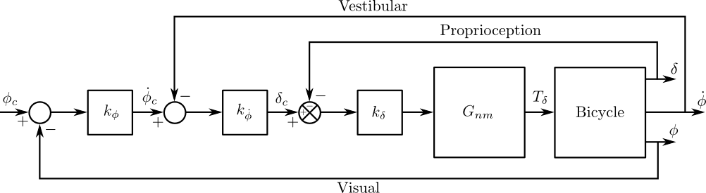
The inner loop structure of the control system which feeds back steer angle \(\delta\), roll rate \(\dot{\phi}\), and roll angle \(\phi\).
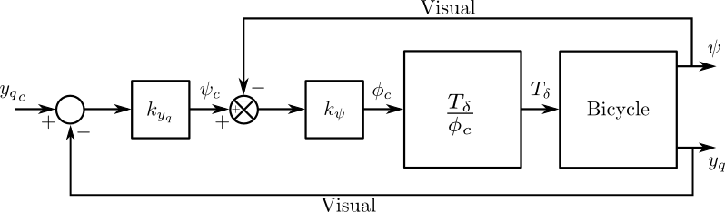
The outer loop structure of the control system with the inner loops closed which feeds back the heading \(\psi\) and the front wheel lateral deviation \(y_q\).
The bicycle block for lateral deviation tracking has states \(x_b = \left[ \phi \quad \delta \quad \dot{\phi} \quad \dot{\delta} \quad \psi \quad y_p \right]^T\), inputs \(u_b = \left[ T_\delta \quad F \right]^T\), and outputs \(y_b = \left[ \delta \quad \phi \quad \dot{\phi} \quad \psi \quad y_q \right]^T\). The state, input, and output matrices are follows
The neuromuscular block is described by the transfer function
which can be written in state space form with the states \(x_{nm} = \left[ T_\delta \quad \dot{T}_\delta \right]^T\), input \(u_{nm} = U_{nm}\) and output \(y_{nm} = T_\delta\).
The combined plant (rider neuromuscular model and bicycle) has states \(x_p = \left[ \phi \quad \delta \quad \dot{\phi} \quad \dot{\delta} \quad \psi \quad y_p \quad T_\delta \quad \dot{T}_\delta \right]^T\), inputs \(u_p = \left[ F \quad U_{nm} \right]^T\), and outputs \(y_p = \left[ \delta \quad \phi \quad \dot{\phi} \quad \psi \quad y_q \right]^T\). The state, input, and output matrices of the plant are
The sequential loop closure rationale dictates that the commanded output variables are
and the input to the neuromuscular block as a function of the desired path is
The input to the neuromuscular block can be written in linear form as
The closed loop state space for lateral deviation tracking can be formed by inserting the controller output \(U_{nm}\) into the plant dynamics \((\mathbf{A}_p,\mathbf{B}_p)\) to rearrange the plant state space to be a function of the desired path and the lateral force, \(u_l = \left[ F \quad y_{qc} \right]^T\). The closed loop system \((\mathbf{A}_p,\mathbf{B}_p)\) takes the same form as the plant system with the exception of the steer torque acceleration equation, which is now a function of the controller gains, the neuromuscular parameters, and the desired path of the front wheel contact point. The new entries to the system matrices are
The output matrix, \(\mathbf{C}_l\), can be constructed to provide any desired outputs, which I choose to be a subset of the outputs we measured during the experiments such as steer angle, roll rate, steer torque, etc.
Given that the bicycle model, \((\mathbf{A}_b,\mathbf{B}_b,\mathbf{C}_b)\), is known, the closed loop analytical state space representation is parameterized by seven parameters: the five controller gains and the two neuromuscular parameters. The model is eighth order with two inputs.
Notice that the controller is unlike a state or output feedback model in the sense that the gains only appear in a single row in the A and B matrices. This reflects some of the inherent limitations the human system has for sensing and actuation. Output feedback systems often require an observer so that full estimated state feedback can be used. This model assumes that the rider does not have that ability. They are only able to sense noisy outputs and adjust their torque compensation within the bandwidth limits of the neuromuscular system based on five simple gains.
I also make use of a second closed loop model which is essentially the same, but the outer lateral deviation tracking loop is removed and tracking a commanded heading remains. This model is seventh order with two inputs.
The numerical values from the model derived from Luke’s runs in the pavilion were used to populate the bicycle state space entries, \((\mathbf{A}_b,\mathbf{B}_b),\mathbf{C}_b)\), except for the entries in the heading and lateral deviation acceleration equations which were calculated with the Whipple model. This has the consequence that those entries are developed with potentially erroneous geometric values such as trail.
Data
Only the runs with lateral disturbances are suitable for identifying the rider controller. I used the subset of 262 valid disturbance runs for the following analysis. This subset included runs from all three riders, both environments, and both the lateral deviation and heading tracking maneuvers. All signals had their means subtracted except for the lateral force.
Identification
In the following analyses the Kalman gain matrix is assumed to be equal to zero and the model takes on an output error form. This was required to bring the number of parameters to a reasonable size and provide a chance at finding the optimal solution.
Through trial and error with many different approaches to identification, I found that finding the optimal solution was not a trivial problem. The SIMO problem with full noise estimation has a minimum of 15 parameters. This problem is fraught with local minima. Even the assumption of an output error structure and the reduction of the parameter space to seven, doesn’t escape the difficulty of finding the true minimum. To have a decent chance at finding a good solution, I opted to identify only the SISO system with the lateral force as the input and the steering angle as the output. The choice of steer angle as the sole output is for much the same reason as in [DL11], i.e. the steer angle is a very good quality measurement and together with steer torque reflects the rider’s contribution to the system dynamics as a reaction to the lateral force.
I used the prediction error method [Lju98] to find the optimal parameters for each run. A good solution required good initial parameter guesses for which I used a combination of stable starting guesses from the loop closure technique described in Chapter Control and recursively used random guesses from previous good and bad solutions as starting points, eventually homing in on the optimal solutions.
The criterion for a good model was based on the variance accounted for in the measurement output. The mean VAF for all the identified runs is \(62 \pm 12\) percent, and considering the large relative human remnant, fits above 30% are still relatively good. I ensured stability in the identified models and no issues associated with unstable simulations corrupting the model quality criteria were present.
It turned out that the identified parameters for the SISO model not only predicted the steer angle, but when extra outputs are added it predicts them well too. The resulting parameters from the SISO model can then be used as initial guesses for the SIMO formulation to check multiple outputs. The identification process followed these steps:
- Process, filter and detrend the data.
- Construct the SISO (Input: \(F\), Output: \(\delta\)) grey box state space model.
- Identify the five gains and the neuromuscular frequency for the lateral force and steer angle data using a variety of initial parameter guesses.
- Construct the SIMO grey box state space model.
- Identify the six parameters as before using the result of the SISO identification as the initial parameter guess for the SIMO system.
The results in Figures 11.22 and 11.23 give typical examples of the model’s ability to predict the measured data in two different runs, one on the treadmill and one on the gymnasium floor, respectively. Notice that the human’s remnant is relatively large when the input is zero, especially in the treadmill run. The model is able to predict the human’s initial control response to the external input and lumps the remnant into the output error. This response is very repeatable across riders and runs. The model considers the remnant as output error during the non perturbed portions of the run. Notice that the steer torque is well predicted around the perturbation. Previous identifications with the Whipple model predicted much lower torque magnitudes and much different parameters. Including the identified bicycle model from Section Canonical Identification proved to give much better control predictions.
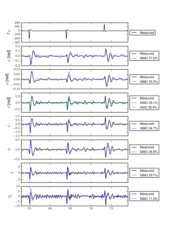
Simulation of an identified model derived from the inputs and outputs (SIMO) of one of Charlie’s treadmill runs #288 (4.23 m/s) validated against the data from run #289 (4.22 m/s). The black line is the processed and filtered (low pass 15 Hz) measured data, the blue line is the simulation from the identified SIMO model and the green line is the identified SISO model. Generated by src/systemidentification/rider_id_model_quality_plot.py.
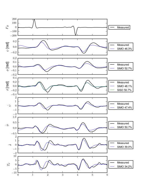
Simulation of an identified model derived from the inputs and outputs (SIMO) of one of Luke’s pavilion runs #657 (3.99 m/s) validated against the data from run #658 (3.74 m/s). The black line is the processed and filtered (low pass 15 Hz) measured data, the blue line is the simulation from the identified SIMO model, and the green line is the identified SISO model. Generated by src/systemidentification/rider_id_model_quality_plot.py.
Results
I computed the optimal five gains and neuromuscular frequency[6] for all 262 runs and recorded the VAF of the steer angle output explained by the model for each run along with the identified parameters.
The first set of quantities of interest are the identified parameters themselves. As I’ve already mentioned in the previous section, identifying the parameters accurately is a function of the number of free parameters, which parameters are free, and the quality of the noise model. In my case, our noise model is an output error structure and may contribute to much more spread in the identified parameters. Figure 11.24 gives an idea of how the six identified parameters vary with speed. As shown in Chapter Control the theory predicts that the gains are mostly linear above about 2 m/s and that the neuromuscular frequency is a constant parameter with respect to the human operator.
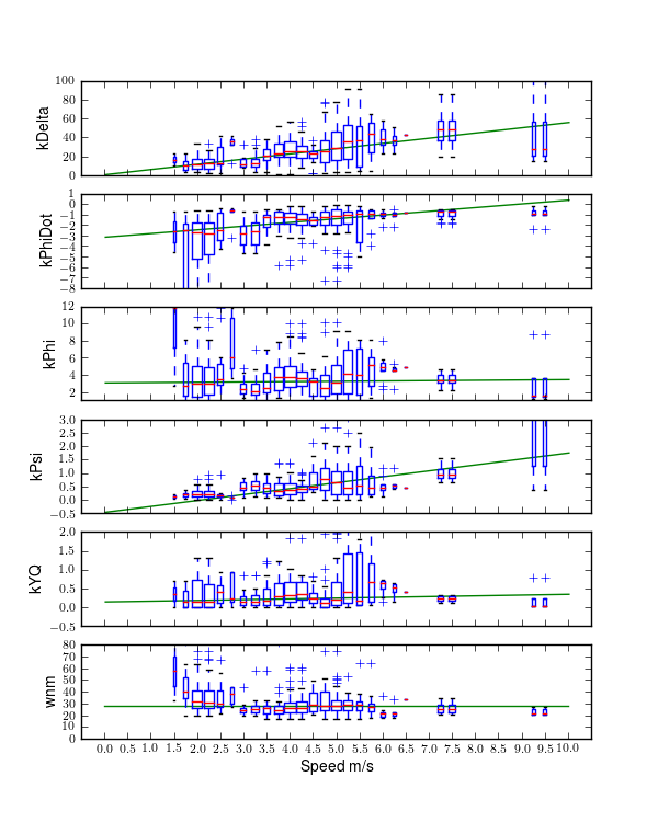
Each of the five identified parameters as a function of speed. The parameter values are grouped into 0.5 m/s speed bins and box plots showing their distributions are given for each speed bin. The red line gives the median of the speed bin, the box bounds the quartiles, and the whisker is 1.5 times the inner quartile range. The width of the boxes are proportional to the square root of the number of runs in the bin. The green line gives the linear fit to the median values which are weighted with respect to the inverse of the standard deviation of each speed bin. The neuromuscular frequency is the best constant that fits the data. Generated by src/systemidentification/control_parameters_vs_speed_plots.py.
Figure 11.24 gives these insights:
- The gains increase with speed with \(k_{\phi}\) and \(k_{y_q}\) having small slopes.
- The low speed runs have much more spread. This is probably due to the fact that the human remnant is relatively large at these speeds and the model attempts to fit the noise rather than casting it as output error.
- The ~9 m/s runs have poorer data quality than other runs due to the treadmill interference in the measurement electronics, thus the spread is large.
- The neuromuscular frequency stays relatively constant just below 30 rad/s, barring the higher variability in the low speed runs.
- The gains may be reasonably characterized with simple linear relationships.
Loop Shaping
The values of the parameters are difficult to directly compare with the ones found by the loop shaping technique described in Chapter Control due to some of the educated guesses about the rider’s internal control choices. But it is possible to evaluate the same loops’ frequency responses in an effort to understand how the rider chooses the gains.
Figure 11.25 shows the frequency response of the closed inner-most loop for a particular speed bin. The theory presented in [HMH12] and Chapter Control postulates that the rider chooses a gain such that the damping ratio of the high frequency neuromuscular peak around 10 rad/s and about gives a 10 dB peak (\(\zeta=0.15\)). Figure 11.25 shows that there may be a more heavily damped neuromuscular peak, but the large variability in the lower frequencies indicates that the rider’s choice is not so constant. This may be explained by the fact that it is more critical for the roll rate loop to exhibit the neuromuscular peaking and the differences in the three rider’s behavior. I’ve previously shown in Chapter Control that there are not necessarily unique gains in the first two loops to achieve the correct peaking in the roll rate loop.
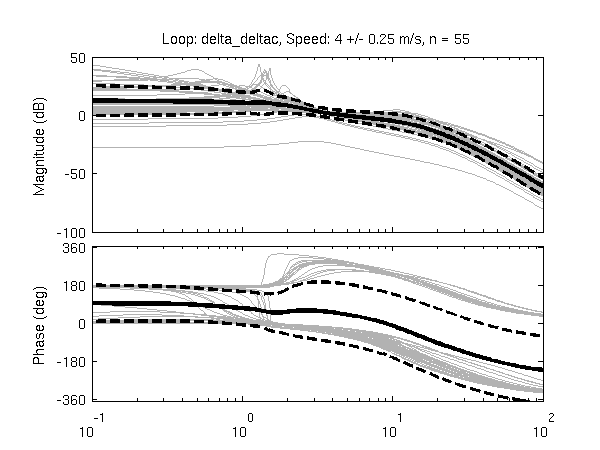
Frequency responses of the closed steer angle loop around 4 m/s. The grey lines plot the response of each individual run in the speed bin while the solid black lines give the mean gain and phase bounded by the dotted black lines which indicate one standard deviation.
Figure 11.26 shows the frequency response of the closed roll rate loop \(\frac{\dot{\phi}}{\dot{\phi}_c}(s)\). As was just pointed out, the theory is that this loop, which completes the inner control loop, must exhibit this typical neuromuscular peaking seen in human-machine control tasks. The mean magnitude plots indicates that this is the case and that the riders do choose their steer and roll rate gains such that the inner loops exhibit the typical response.
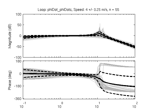
Frequency responses of the closed roll rate loop around 4 m/s. The grey lines plot the response of each individual run in the speed bin while the solid black line give the mean gain and phase bounded by the dotted black lines which indicate the one sigma standard deviation.
Our theory for the selection of the remaining three gains suggests that the loops follow the dictates of the crossover model (i.e. 20 db slope around crossover) and that the crossover frequencies start at 2 and each successive loop is closed at half the previous crossover frequency such that the roll angle, heading and lateral deviation loops are closed in that order. Figures 11.27, 11.28, and 11.29 show the empirically derived frequency responses for the remaining loops.
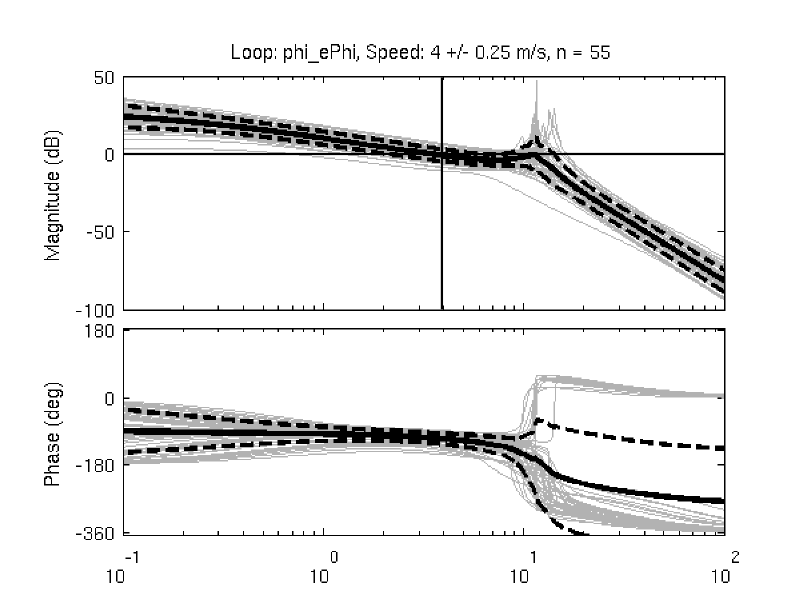
Frequency responses of the open roll angle loop around 4 m/s. The grey lines plot the response of each individual run in the speed bin while the solid blacks line give the mean gain and phase bounded by the dotted black lines which indicate one standard deviation.
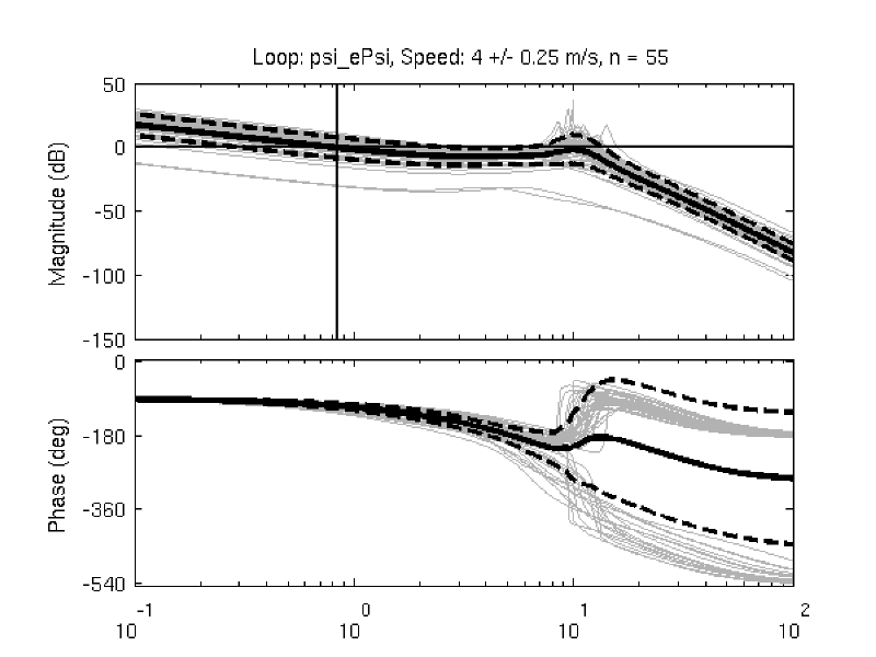
Frequency responses of the open heading loop around 4 m/s. The grey lines plot the response of each individual run in the speed bin while the solid blacks line give the mean gain and phase bounded by the dotted black lines which indicate one standard deviation.
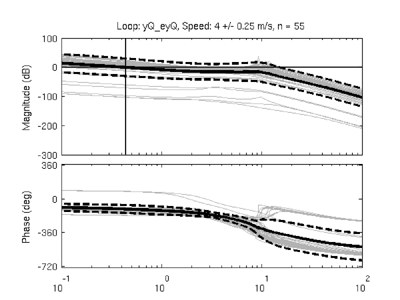
Frequency responses of the open lateral deviation loop around 4 m/s. The grey lines plot the response of each individual run in the speed bin while the solid black lines give the mean gain and phase bounded by the dotted black lines which indicate one standard deviation.
The median crossover frequencies for this 4 m/s speed bin are \(\omega_{\phi c}=3.66\), \(\omega_{\psi c}= 0.98\), and \(\omega_{y_q c}=1.06\). This indicates that the rider is more aggressive than our theory predicts with the higher roll crossover frequency in the roll angle loop. Also, the riders do not crossover at half the previous frequency, with the two outer loops crossing over at about the same frequency indicating that the lateral deviation tracking is more pertinent to the rider than the theory suggests. This may be partially due to the narrowness of the treadmill which constitutes 80% of the data.
Our hypothesis is that the crossover frequencies are constant with respect to speed, so the distribution of the crossover frequencies for all runs should have a tight distribution regardless of speed. Secondly, we postulated that the rider crosses over the roll angle loop around 2 rad/s. Figure 11.30 shows the distribution of the crossover frequencies for each loop where the median values of the crossover frequencies are \(w_{\phi c}=3.31\), \(w_{\psi c}= 1.20\), and \(w_{y_q c}=0.98\), all with somewhat large standard deviations.
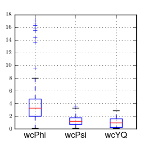
Median crossover frequencies in rad/s for the open outer loops for all runs at all speeds.
If the medians are any indication of the true crossover frequency the rider is more aggressive than predicted and the two outer loop crossover frequencies are much closer in value than predicted. The one-half rule of thumb does seem to hold for the inner two loops.
Full System Response
Once the loops are all closed the system output response to the two inputs \(F_B\) and \(y_{qc}\) can be examined. Given a commanded input \(y_{qc}\), the tracking performance can be gauged by the closed loop Bode plot \(\frac{y_q}{y_{qc}}(s)\) given in Figure 11.31. Notice that in general, the response is well behaved with a 0 dB magnitude out to about 10 rad/s, all poles are stable and the phase lag increases gradually with frequency.

Frequency responses of the closed loop system lateral deviation tracking response around 4 m/s. The grey lines plot the response of each individual run in the speed bin while the solid black lines give the mean gain and phase bounded by the dotted black lines which indicate one standard deviation.
Similarly, the system’s response to the lateral disturbance force Figure 11.32 is favorable for all the identified models and shows good disturbance rejection.
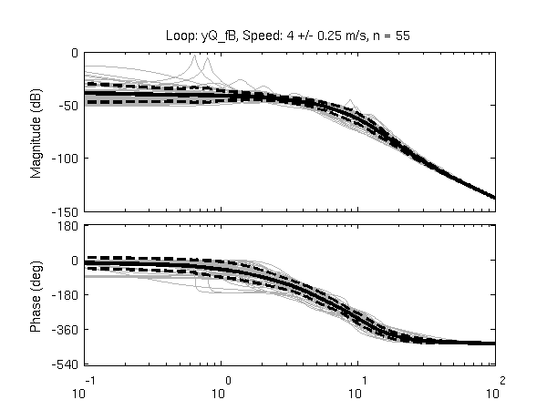
Frequency responses of the closed loop system disturbance rejection response around 4 m/s. The grey lines plot the response of each individual run in the speed bin while the solid black lines give the mean gain and phase bounded by the dotted black lines which indicate one standard deviation.
The reader may note that some of the Bode plots among Figures 11.25-11.29 indicate instability in that amplitude and phase characteristics synonymous with quadratic poles with small, positive damping ratios are in evidence. For example, one can see the evidence of such poles around 1-2 rad/s in Figure 11.25 and 10 rad/s in Figure 11.26. It should be emphasized that these Bode plots represent either (1) open-loop transfer functions, or (2) inner, closed loop transfer functions. Hence, they do not imply final, outer closed loop instabilities. Indeed, the Bode plots of the outer-most, closed loop transfer function of Figure 11.31 (lateral deviation) do not indicate any such quadratic poles with small positive damping ratios. The gain selection procedure in Chapter Control attempted to insure stability at least by closing of the roll angle loop, but these plots show that may not always be required for adequate performance for the complete system.
Conclusion
I have shown that a simple rider controller can be identified from the collected data given that the plant model of the bicycle/rider system is properly chosen, in my case identified separately from the same data. In addition these basic conclusion arise:
- The fundamental, remnant-free, control response of the rider under lateral perturbations can be described reasonably well by the simple five gain sequential loop closure and an eighth order closed loop system. No time delays are needed and the continuous formulation is adequate for good prediction.
- The identified gains seem to exhibit linear trends with respect to speed as predicted by theory and the identified neuromuscular frequency seems to be constant with a median around the theoretical prediction of 30 rad/s.
- The identified parameters show resemblance to the patterns in the theoretical loop closure techniques, especially in that the rider selects their gains such that the closed roll rate loop exhibits a 10 dB peak around 10-11 rad/s and that the riders cross over the outer three loops in the predicted order.
- The crossover frequencies of the three outer loops are relatively constant with respect to speed and point to a speed independence of system response bandwidth selection among riders in this task.
- The parameters do not seem to be uniquely identified if the neuromuscular damping ratio is included as a free parameter.
All of these conclusions are based on a preliminary statistical view of the data. I believe the spread in the results can be tightened up significantly with further data processing and the use of both simple and more complex statistical methods. In my view, the data set still has a lot more tell with further analysis but it has also revealed the need for further simplified experiments. The following are some thoughts on improving the analysis:
- Improving the bicycle model.
- To have any hope of identifying a realistic and accurate controller, the plant must have a very good representative model. The bicycle is an excellent platform for testing the human’s control system due to it’s low speed instability and the fact that non-trivial control is needed to stabilize and direct the non-minimum phase system, but the first principles models for bicycle/rider biomechanics are not yet adequate or descriptive enough to describe the plant. This is mostly due to poor understanding of the tire to ground interaction and the rider’s complicated coupling to the bicycle frames in which the rider is free to use more than one actuation for control. But, as has been shown here, system identification can be used to develop a realistic plant model for specific bicycles and even small variations in riders. A data driven model is currently the best choice until the first principles models are able to catch up and may, in fact, be able to provide more robust models due to the inherent complexity of describing all of the system with first principles.
- Estimating the process noise matrix.
- The better one can estimate the process noise in the system, the more accurate the parameter predictions will get. In all of my attempts I had little success in ever estimating the optimal model when some or all of the process noise parameters were free. For the controller portion, the process noise is not awfully different in magnitudes than the rider’s control actions with respect to the disturbance and it is very apparent in the low speed runs. This type of noise is much more difficult to properly account for. The parameter estimates from the output error structures used in this study are susceptible to the model fitting the noise and the control actions as opposed to just the control actions. The identifications fortunately were able to fit the control actions and not the noise and this is much more apparent and true in the treadmill runs. It may be possible to develop estimates of the process and measurement noise covariance matrices from the undisturbed runs where the human’s remnant is the dominant source of variability in the outputs.
- Fixing the neuromuscular model.
- The results give some indication that the neuromuscular model is an appropriate choice. The gain identification could possibly be improved by fixing both the neuromuscular frequency and damping ratio, and only estimating the gains. In general, the more parameters you can be confident about via first principles, the more the identified parameters may be able to tell you about the system with higher certainty.
- Removing outliers.
- A more systematic approach to the removal of outlier data using criteria from the resulting fit variance, parameters, and frequency responses would help tighten up the data. The outliers are quite apparent in the data I’ve shown and a detailed look at why they are outliers may allow many of them to be removed.
- Mixed effects modeling.
- There are statistical methods available that can account for all of the factors and repeated experiments. One such method is mixed effects or multilevel modeling. I explored the use of these in a preliminary fashion but need more time to understand the methods so that I apply them correctly. This would provide models based on the many factors in the experiments and give stronger comparisons with respect to them, such as variations among riders and environments.
- First Principles Checks
- There are potentially some simpler checks that can be run with respect to the first principles models. For example, the Whipple equations of motion can be formulated with no nonholonomic lateral and longitudinal wheel constraints leaving only unknown tire forces. The data I’ve collected, in particular the lateral accelerations and roll, yaw, steer angles and rates, can be used to calculate the in-ground-plane forces at the tire contact points. If these forces aren’t the same as the nonholonomic constraints predict, then tire slip must be occurring. This validation and others can be performed with the data set I’ve collected, potentially answering some important questions.
If I had unlimited time, I would work on these ideas more thoroughly. I hope to be able to explore the data in more detail with better methodologies and ideas in the future, but that may or may not happen. Fortunately the data is available if others would like to try out different methods, plant models, bicycle models, etc. and my methods, software, and methodologies are hopefully detailed enough for reuse.
Footnotes
| [1] | First principles here means any modeling techniques that use fundamental “known” building blocks to create a dynamic model. These buildling blocks can include items such as Newton’s laws of motion, the laws of thermodynamics, friction and contact models, electrical components, etc. |
| [2] | This overdamped low bandwidth neuromuscular model is very different than what we assumed and ultimately identified. |
| [3] | The floor is a product called “pulastic” which is manufactured by Robbins Sport Surfaces. |
| [4] | I spent some time trying to regress models to each of the speed dependent coefficients in the state space model by assuming either a constant, linear, or quadratic line. I tried simple regression techniques and also some mixed effects techniques to obviate the fact that some of the speed bins had many more runs than others. This method may be used to generate a speed independent model based on all of the runs, but needs more work. |
| [5] | It is also possible to solve the roll and steer equations simultaneously and enforce the symmetry, which is probably a better idea. |
| [6] | The nueromuscaulr damping ratio was fixed to 0.707 as per [MM71]. The uniqueness of the identifiablity of the parameters is questionable if this is not fixed, as wildly different solutions for the neuromuscular frequency were often found if the damping ratio was left free. |
