Energy and Power

Note

You can download this example as a Python script: energy.py or Jupyter Notebook: energy.ipynb.

from IPython.display import HTML
from matplotlib.animation import FuncAnimation
from scikits.odes import dae
from scipy.optimize import fsolve
import matplotlib.pyplot as plt
import numpy as np
import sympy as sm
import sympy.physics.mechanics as me
me.init_vprinting(use_latex='mathjax')

class ReferenceFrame(me.ReferenceFrame):

    def __init__(self, *args, **kwargs):

        kwargs.pop('latexs', None)

        lab = args[0].lower()
        tex = r'\hat{{{}}}_{}'

        super(ReferenceFrame, self).__init__(*args,
                                             latexs=(tex.format(lab, 'x'),
                                                     tex.format(lab, 'y'),
                                                     tex.format(lab, 'z')),
                                             **kwargs)
me.ReferenceFrame = ReferenceFrame

Learning Objectives

After completing this chapter readers will be able to:

• calculate the kinetic and potential energy of a multibody system

• evaluate a simulation for energy gains and losses

Introduction

So far we have investigated multibody systems from the perspective of forces and their relationship to motion. It is also useful to understand these systems from a power and energy perspective. Power \(P\) is the time rate of change in work \(W\) done where work is the energy gained, dissipated, or exchanged in a system.

(216)\[P = \frac{\text{d}W}{\text{d}t}\]

Conversely, work is the integral of power:

(217)\[W(t) = \int_{t_0}^{t_f} P(t) \text{d}t\]

The work done by a force \(\bar{F}\) acting on a point located by position vector \(\bar{r}(t)\) is calculated as:

(218)\[W = \int_{\bar{r}(t_0)}^{\bar{r}(t_1)}\bar{F}\cdot \text{d}\bar{r} = \int_{t_0}^{t_1}\bar{F}\cdot \dot{\bar{r}} \text{d}t\]

From which we also see \(P = \bar{F}\cdot \dot{\bar{r}}\).

Energy in a multibody system comes in many forms and can be classified as kinetic, potential (conservative), or non-conservative. Any energy that enters or leaves the system is non-conservative.

Kinetic Energy

Kinetic energy \(K\) is an instantaneous measure of the energy due to motion of all of the particles and rigid bodies in a system. A rigid body will, in general, have a translational and a rotational component of kinetic energy. A particle cannot rotate so it only has translational kinetic energy. Kinetic energy can be thought of as the work done by the generalized inertia forces \(\bar{F}^*_r\) with going from the current state to rest.

Translational kinetic energy of a particle \(Q\) of mass \(m\) in reference frame \(N\) is:

(219)\[K_Q := \frac{1}{2}m\left|{}^N\bar{v}^{Q}\right|^2 = \frac{1}{2}m {}^N\bar{v}^{Q} \cdot {}^N\bar{v}^{Q}\]

If \(Q\) is the mass center of a rigid body, the equation represents the translational kinetic energy of the rigid body. The rotational kinetic energy of a rigid body \(B\) with mass center \(B_o\) in \(N\) is added to its translational kinetic energy and the total kinetic energy of \(B\) is defined as:

(220)\[K_B := \frac{1}{2} m {}^N\bar{v}^{B_o} \cdot {}^N\bar{v}^{B_o} + \frac{1}{2} {}^N\bar{\omega}^B \cdot \breve{I}^{B/B_o} \cdot {}^N\bar{\omega}^B\]

The total kinetic energy in a multibody system is the sum of the kinetic energies for all particles and rigid bodies.

Potential Energy

Some of the generalized active force contributions in inertial reference frame \(N\) can be written as

(221)\[F_r = -\frac{\partial V}{\partial q_r}\]

when \(\bar{u}=\dot{\bar{q}}\) and where \(V\) is strictly a function of the generalized coordinates and time, i.e. \(V(\bar{q}, t)\). These functions \(V\) are potential energies in \(N\). The associated generalized active force contributions are from conservative forces. They are forces for which the work done by the force for any path \(\bar{r}(t)\) starting and ending at the same position equals zero. The most common conservative forces seen in multibody systems are gravitational forces and ideal spring forces, but there are conservative forces related to electrostatic forces, magnetic forces, etc.

For small objects at Earth’s surface we model gravity as a uniform field and the potential energy of a particle or rigid body is:

(222)\[V = mgh\]

where \(m\) is the body or particle’s mass, \(g\) is the acceleration due to gravity at the Earth’s surface, and \(h(\bar{q}, t)\) is the distance parallel to the gravitational field direction of the particle or body with respect to an arbitrary reference point.

A linear spring generates a conservative force \(F=kx\) between two points \(P\) and \(Q\) and its potential energy is:

(223)\[V_s = \frac{1}{2} k \left| \bar{r}^{P/Q} \right|^2 = \frac{1}{2} k \bar{r}^{P/Q} \cdot \bar{r}^{P/Q}\]

The sum of all potential energies in a system give the total potential energy of the system.

Total Energy

The total energy of the system is:

(224)\[E := K + V\]

If \(\bar{F}_r\) is only made up of conservative forces, then the system is conservative and will not lose energy as it moves, it simply exchanges kinetic for potential and vice versa, i.e. \(E\) is constant for conservative systems.

Energetics of Jumping

Let’s create a simple multibody model of a person doing a vertical jump like shown in the video below so that we can calculate the kinetic and potential energy.

We can model the jumper in a single plane with two rigid bodies representing the thigh \(B\) and the calf \(A\) of the legs lumping the left and right leg segments together. The mass centers of the leg segments lie on the line connecting the segment end points but at some distance from the ends \(d_a,d_b\). To avoid having to stabilize the jumper, we can assume that particles representing the foot \(P_f\) and the upper body \(P_u\) can only move vertically and are always aligned vertically over one another. The foot \(P_f\), knee \(P_k\), and hip \(P_u\) are all modeled as pin joints. The mass of the foot \(m_f\) and the mass of the upper body are modeled as particles at \(P_f\) and \(P_u\), respectively. We will model a collision force \(F_f\) from the ground \(N\) acting on the foot \(P_f\) using the Hunt-Crossley formulation described in Collision. We will actuate the jumper using only a torque acting between the thigh and the calf \(T_k\) that represents the combine forces of the muscles attached between the two leg segments. Fig. 52 shows a free body diagram of the model.

Fig. 52 Free body diagram of a simple model of a human jumper.

Equations of Motion

We first define all of the necessary symbols:

g = sm.symbols('g')
mu, ma, mb, mf = sm.symbols('m_u, m_a, m_b, m_f')
Ia, Ib = sm.symbols('I_a, I_b')
kf, cf, kk, ck = sm.symbols('k_f, c_f, k_k, c_k')
la, lb, da, db = sm.symbols('l_a, l_b, d_a, d_b')

q1, q2, q3 = me.dynamicsymbols('q1, q2, q3', real=True)
u1, u2, u3 = me.dynamicsymbols('u1, u2, u3', real=True)
Tk = me.dynamicsymbols('T_k')

t = me.dynamicsymbols._t

q = sm.Matrix([q1, q2, q3])
u = sm.Matrix([u1, u2, u3])
ud = u.diff(t)
us = sm.Matrix([u1, u3])
usd = us.diff(t)
p = sm.Matrix([
    Ia,
    Ib,
    cf,
    ck,
    da,
    db,
    g,
    kf,
    kk,
    la,
    lb,
    ma,
    mb,
    mf,
    mu,
])
r = sm.Matrix([Tk])

Then we set up the kinematics:

N = me.ReferenceFrame('N')
A = me.ReferenceFrame('A')
B = me.ReferenceFrame('B')

A.orient_axis(N, q2, N.z)
B.orient_axis(A, q3, N.z)

A.set_ang_vel(N, u2*N.z)
B.set_ang_vel(A, u3*N.z)

O = me.Point('O')
Ao, Bo = me.Point('A_o'), me.Point('B_o')
Pu, Pk, Pf = me.Point('P_u'), me.Point('P_k'), me.Point('P_f')

Pf.set_pos(O, q1*N.y)
Ao.set_pos(Pf, da*A.x)
Pk.set_pos(Pf, la*A.x)
Bo.set_pos(Pk, db*B.x)
Pu.set_pos(Pk, lb*B.x)

O.set_vel(N, 0)
Pf.set_vel(N, u1*N.y)
Pk.v2pt_theory(Pf, N, A)
Pu.v2pt_theory(Pk, N, B)

qd_repl = {q1.diff(t): u1, q2.diff(t): u2, q3.diff(t): u3}
qdd_repl = {q1.diff(t, 2): u1.diff(t), q2.diff(t, 2): u2.diff(t), q3.diff(t, 2): u3.diff(t)}

holonomic = Pu.pos_from(O).dot(N.x)
vel_con = holonomic.diff(t).xreplace(qd_repl)
acc_con = vel_con.diff(t).xreplace(qdd_repl).xreplace(qd_repl)

# q2 is dependent

u2_repl = {u2: sm.solve(vel_con, u2)[0]}
u2d_repl = {u2.diff(t): sm.solve(acc_con, u2.diff(t))[0].xreplace(u2_repl)}

Gravity acts on all the masses and mass centers and we have a single force acting on the foot from the ground that includes the collision stiffness and damping terms with coefficients \(k_f\) and \(c_f\) respectively.

R_Pu = -mu*g*N.y
R_Ao = -ma*g*N.y
R_Bo = -mb*g*N.y

zp = (sm.Abs(q1) - q1)/2
damping = sm.Piecewise((-cf*u1, q1<0), (0.0, True))
Ff = (kf*zp**(sm.S(3)/2) + damping)*N.y

R_Pf = -mf*g*N.y + Ff
R_Pf

\[\begin{split}\displaystyle (- g m_{f} + k_{f} \left(- \frac{q_{1}}{2} + \frac{\left|{q_{1}}\right|}{2}\right)^{\frac{3}{2}} + \begin{cases} - c_{f} u_{1} & \text{for}\: q_{1} < 0 \\0.0 & \text{otherwise} \end{cases})\hat{n}_y\end{split}\]

The torques on the thigh and calf will include a passive stiffness and damping to represent muscle tendons and tissue effects with coefficients \(k_k\) and \(c_k\) respectively as well as the muscle actuation torque \(T_k\).

T_A = (kk*(q3 - sm.pi/2) + ck*u3 + Tk)*N.z
T_B = -T_A
T_A

\[\displaystyle (c_{k} u_{3} + k_{k} \left(q_{3} - \frac{\pi}{2}\right) + T_{k})\hat{n}_z\]

Define the inertia dyadics for the legs:

I_A_Ao = Ia*me.outer(N.z, N.z)
I_B_Bo = Ib*me.outer(N.z, N.z)

Finally, formulate Kane’s equations:

points = [Pu, Ao, Bo, Pf]
forces = [R_Pu, R_Ao, R_Bo, R_Pf]
masses = [mu, ma, mb, mf]

frames = [A, B]
torques = [T_A, T_B]
inertias = [I_A_Ao, I_B_Bo]

Fr_bar = []
Frs_bar = []

for ur in [u1, u3]:

   Fr = 0
   Frs = 0

   for Pi, Ri, mi in zip(points, forces, masses):
      N_v_Pi = Pi.vel(N).xreplace(u2_repl)
      vr = N_v_Pi.diff(ur, N)
      Fr += vr.dot(Ri)
      N_a_Pi = Pi.acc(N).xreplace(u2d_repl).xreplace(u2_repl)
      Rs = -mi*N_a_Pi
      Frs += vr.dot(Rs)

   for Bi, Ti, Ii in zip(frames, torques, inertias):
      N_w_Bi = Bi.ang_vel_in(N).xreplace(u2_repl)
      N_alp_Bi = Bi.ang_acc_in(N).xreplace(u2d_repl).xreplace(u2_repl)
      wr = N_w_Bi.diff(ur, N)
      Fr += wr.dot(Ti)
      Ts = -(N_alp_Bi.dot(Ii) + me.cross(N_w_Bi, Ii).dot(N_w_Bi))
      Frs += wr.dot(Ts)

   Fr_bar.append(Fr)
   Frs_bar.append(Frs)

Fr = sm.Matrix(Fr_bar)
Frs = sm.Matrix(Frs_bar)
kane_eq = Fr + Frs

Energy

The total potential energy is derived based on the height of all the particles and rigid body mass centers above a reference point \(O\) on the ground and the two springs: passive knee stiffness and the ground-foot stiffness. The work done by these two springs can be found using integrate():

Vf = -sm.integrate(kf*zp**(sm.S(3)/2), q1)
Vf

\[\begin{split}\displaystyle - \begin{cases} 0 & \text{for}\: q_{1} \geq 0 \\- \frac{2 k_{f} \left(- q_{1}\right)^{\frac{5}{2}}}{5} & \text{otherwise} \end{cases}\end{split}\]

Vk = sm.integrate(kk*(q3 - sm.pi/2), q3)
Vk

\[\displaystyle \frac{k_{k} q_{3}^{2}}{2} - \frac{\pi k_{k} q_{3}}{2}\]

V = (
    (mf*g*Pf.pos_from(O) +
     ma*g*Ao.pos_from(O) +
     mb*g*Bo.pos_from(O) +
     mu*g*Pu.pos_from(O)).dot(N.y) +
    Vf + Vk
)
V

\[\begin{split}\displaystyle g m_{a} q_{1} + g m_{b} q_{1} + g m_{f} q_{1} + g m_{u} q_{1} + \frac{k_{k} q_{3}^{2}}{2} - \frac{\pi k_{k} q_{3}}{2} + \left(\sin{\left(q_{2} \right)} \cos{\left(q_{3} \right)} + \sin{\left(q_{3} \right)} \cos{\left(q_{2} \right)}\right) \left(d_{b} g m_{b} + g l_{b} m_{u}\right) + \left(d_{a} g m_{a} + g l_{a} m_{b} + g l_{a} m_{u}\right) \sin{\left(q_{2} \right)} - \begin{cases} 0 & \text{for}\: q_{1} \geq 0 \\- \frac{2 k_{f} \left(- q_{1}\right)^{\frac{5}{2}}}{5} & \text{otherwise} \end{cases}\end{split}\]

The kinetic energy is made up of the translational kinetic energy of the foot and upper body particles \(K_f\) and \(K_u\):

Kf = mf*me.dot(Pf.vel(N), Pf.vel(N))/2
Ku = mu*me.dot(Pu.vel(N), Pu.vel(N))/2
Kf, sm.simplify(Ku)

\[\displaystyle \left( \frac{m_{f} u_{1}^{2}}{2}, \ \frac{m_{u} \left(l_{a}^{2} u_{2}^{2} + 2 l_{a} l_{b} \left(u_{2} + u_{3}\right) u_{2} \cos{\left(q_{3} \right)} + 2 l_{a} u_{1} u_{2} \cos{\left(q_{2} \right)} + l_{b}^{2} \left(u_{2} + u_{3}\right)^{2} + 2 l_{b} \left(u_{2} + u_{3}\right) u_{1} \cos{\left(q_{2} + q_{3} \right)} + u_{1}^{2}\right)}{2}\right)\]

as well as the translational and rotational kinetic energies of the calf and thigh \(K_A\) and \(K_B\):

KA = ma*me.dot(Ao.vel(N), Ao.vel(N))/2 + me.dot(me.dot(A.ang_vel_in(N), I_A_Ao), A.ang_vel_in(N))/2
KA

\[\displaystyle \frac{I_{a} u_{2}^{2}}{2} + \frac{m_{a} \left(d_{a}^{2} u_{2}^{2} + 2 d_{a} u_{1} u_{2} \cos{\left(q_{2} \right)} + u_{1}^{2}\right)}{2}\]

KB = mb*me.dot(Bo.vel(N), Bo.vel(N))/2 + me.dot(me.dot(B.ang_vel_in(N), I_B_Bo), B.ang_vel_in(N))/2
sm.simplify(KB)

\[\displaystyle \frac{I_{b} \left(u_{2} + u_{3}\right)^{2}}{2} + \frac{m_{b} \left(d_{b}^{2} \left(u_{2} + u_{3}\right)^{2} + 2 d_{b} l_{a} \left(u_{2} + u_{3}\right) u_{2} \cos{\left(q_{3} \right)} + 2 d_{b} \left(u_{2} + u_{3}\right) u_{1} \cos{\left(q_{2} + q_{3} \right)} + l_{a}^{2} u_{2}^{2} + 2 l_{a} u_{1} u_{2} \cos{\left(q_{2} \right)} + u_{1}^{2}\right)}{2}\]

The total kinetic energy of the system is then \(K=K_f+K_u+K_A+K_B\):

K = Kf + Ku + KA + KB

Simulation Setup

We will simulate the system to investigate the energy. Below are various functions that convert the symbolic equations to numerical functions, simulate the system with some initial conditions, and plot/animate the results. These are similar to prior chapters, so I leave them unexplained.

Simulation code

eval_kane = sm.lambdify((q, usd, us, r, p), kane_eq)
eval_holo = sm.lambdify((q, p), holonomic)
eval_vel_con = sm.lambdify((q, u, p), vel_con)
eval_acc_con = sm.lambdify((q, ud, u, p), acc_con)
eval_energy = sm.lambdify((q, us, p), (K.xreplace(u2_repl), V.xreplace(u2_repl)))

coordinates = Pf.pos_from(O).to_matrix(N)
for point in [Ao, Pk, Bo, Pu]:
   coordinates = coordinates.row_join(point.pos_from(O).to_matrix(N))
eval_point_coords = sm.lambdify((q, p), coordinates)

def eval_eom(t, x, xd, residual, p_r):
    """Returns the residual vector of the equations of motion.

    Parameters
    ==========
    t : float
       Time at evaluation.
    x : ndarray, shape(5,)
       State vector at time t: x = [q1, q2, q3, u1, u3].
    xd : ndarray, shape(5,)
       Time derivative of the state vector at time t: xd = [q1d, q2d, q3d, u1d, u3d].
    residual : ndarray, shape(5,)
       Vector to store the residuals in: residuals = [fk, fd, fh].
    r : function
      Function of [Tk] = r(t, x) that evaluates the input Tk.
    p : ndarray, shape(15,)
       Constant parameters: p = [Ia, Ib, cf, ck, da, db, g, kf, kk, la, lb,
       ma, mb, mf, mu]

    """

    p, r = p_r

    q1, q2, q3, u1, u3 = x
    q1d, _, q3d, u1d, u3d = xd  # ignore the q2d value

    residual[0] = -q1d + u1
    residual[1] = -q3d + u3
    residual[2:4] = eval_kane([q1, q2, q3], [u1d, u3d], [u1, u3], r(t, x, p), p).squeeze()
    residual[4] = eval_holo([q1, q2, q3], p)

def setup_initial_conditions(q1, q3, u1, u3):

   q0 = np.array([q1, np.nan, q3])

   q0[1] = fsolve(lambda q2: eval_holo([q0[0], q2, q0[2]], p_vals),
                  np.deg2rad(45.0))[0]

   u0 = np.array([u1, u3])

   u20 = fsolve(lambda u2: eval_vel_con(q0, [u0[0], u2, u0[1]], p_vals),
                np.deg2rad(0.0))[0]

   x0 = np.hstack((q0, u0))

   # TODO : use equations to set these
   ud0 = np.array([0.0, 0.0])

   xd0 = np.hstack(([u0[0], u20, u0[1]], ud0))

   return x0, xd0

def simulate(t0, tf, fps, x0, xd0, p_vals, eval_r):

   ts = np.linspace(t0, tf, num=int(fps*(tf - t0)))

   solver = dae('ida',
                eval_eom,
                rtol=1e-8,
                atol=1e-8,
                algebraic_vars_idx=[4],
                user_data=(p_vals, eval_r),
                old_api=False)

   solution = solver.solve(ts, x0, xd0)

   ts = solution.values.t
   xs = solution.values.y

   Ks, Vs = eval_energy(xs[:, :3].T, xs[:, 3:].T, p_vals)
   Es = Ks + Vs

   Tks = np.empty_like(ts)
   for i, ti in enumerate(ts):
       Tks[i] = eval_r(ti, None, None)[0]

   return ts, xs, Ks, Vs, Es, Tks

def plot_results(ts, xs, Ks, Vs, Es, Tks):
    """Returns the array of axes of a 4 panel plot of the state trajectory
    versus time.

    Parameters
    ==========
    ts : array_like, shape(n,)
       Values of time.
    xs : array_like, shape(n, 4)
       Values of the state trajectories corresponding to ``ts`` in order
       [q1, q2, q3, u1, u3].

    Returns
    =======
    axes : ndarray, shape(3,)
       Matplotlib axes for each panel.

    """
    fig, axes = plt.subplots(6, 1, sharex=True)

    fig.set_size_inches((10.0, 6.0))

    axes[0].plot(ts, xs[:, 0])  # q1(t)
    axes[1].plot(ts, np.rad2deg(xs[:, 1:3]))  # q2(t), q3(t)
    axes[2].plot(ts, xs[:, 3])  # u1(t)
    axes[3].plot(ts, np.rad2deg(xs[:, 4]))  # u3(t)
    axes[4].plot(ts, Ks)
    axes[4].plot(ts, Vs)
    axes[4].plot(ts, Es)
    axes[5].plot(ts, Tks)

    axes[0].legend(['$q_1$'])
    axes[1].legend(['$q_2$', '$q_3$'])
    axes[2].legend(['$u_1$'])
    axes[3].legend(['$u_3$'])
    axes[4].legend(['$K$', '$V$', '$E$'])
    axes[5].legend(['$T_k$'])

    axes[0].set_ylabel('Distance [m]')
    axes[1].set_ylabel('Angle [deg]')
    axes[2].set_ylabel('Speed [m/s]')
    axes[3].set_ylabel('Angular Rate [deg/s]')
    axes[4].set_ylabel('Energy [J]')
    axes[5].set_ylabel('Torque [N-m]')
    axes[5].set_xlabel('Time [s]')

    fig.tight_layout()

    return axes

def setup_animation_plot(ts, xs, p):
    """Returns objects needed for the animation.

    Parameters
    ==========
    ts : array_like, shape(n,)
       Values of time.
    xs : array_like, shape(n, 4)
       Values of the state trajectories corresponding to ``ts`` in order
       [q1, q2, q3, u1].
    p : array_like, shape(?,)

    """

    x, y, _ = eval_point_coords(xs[0, :3], p)

    fig, ax = plt.subplots()
    fig.set_size_inches((10.0, 10.0))
    ax.set_aspect('equal')
    ax.grid()

    lines, = ax.plot(x, y, color='black',
                     marker='o', markerfacecolor='blue', markersize=10)

    title_text = ax.set_title('Time = {:1.1f} s'.format(ts[0]))
    ax.set_xlim((-0.5, 0.5))
    ax.set_ylim((0.0, 1.5))
    ax.set_xlabel('$x$ [m]')
    ax.set_ylabel('$y$ [m]')
    ax.set_aspect('equal')

    return fig, ax, title_text, lines

def animate_linkage(ts, xs, p):
    """Returns an animation object.

    Parameters
    ==========
    ts : array_like, shape(n,)
    xs : array_like, shape(n, 4)
       x = [q1, q2, q3, u1]
    p : array_like, shape(6,)
       p = [la, lb, lc, ln, m, g]

    """
    # setup the initial figure and axes
    fig, ax, title_text, lines = setup_animation_plot(ts, xs, p)

    # precalculate all of the point coordinates
    coords = []
    for xi in xs:
        coords.append(eval_point_coords(xi[:3], p))
    coords = np.array(coords)

    # define the animation update function
    def update(i):
        title_text.set_text('Time = {:1.1f} s'.format(ts[i]))
        lines.set_data(coords[i, 0, :], coords[i, 1, :])

    # close figure to prevent premature display
    plt.close()

    # create and return the animation
    return FuncAnimation(fig, update, len(ts))

Conservative Simulation

For the first simulation, let’s disable the ground reaction force and the passive and active knee behavior and simply let the leg fall in space.

p_vals = np.array([
  0.101,  # Ia,
  0.282,  # Ib,
  0.0,    # cf,
  0.0,    # ck,
  0.387,  # da,
  0.193,  # db,
  9.81,   # g,
  0.0,    # kf,
  0.0,    # kk,
  0.611,  # la,
  0.424,  # lb,
  6.769,  # ma,
  17.01,  # mb,
  3.0,    # mf,
  32.44,  # mu
])

x0, xd0 = setup_initial_conditions(0.2, np.deg2rad(20.0), 0.0, 0.0)

def eval_r(t, x, p):
   return [0.0]  # [Tk]

t0, tf, fps = 0.0, 0.5, 30
ts_dae, xs_dae, Ks, Vs, Es, Tks = simulate(t0, tf, fps, x0, xd0, p_vals, eval_r)

HTML(animate_linkage(ts_dae, xs_dae, p_vals).to_jshtml(fps=fps))

Once Loop Reflect

plot_results(ts_dae, xs_dae, Ks, Vs, Es, Tks);

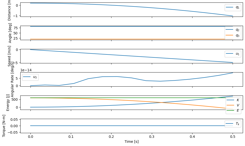
With no dissipation and only conservative forces acting on the system (gravity), the total energy \(E\) should stay constant, which it does. Checking whether energy remains constant is a useful for sussing out whether your model is likely valid. So far so good for us.

Conservative Simulation with Ground Spring

For the second simulation of this model we will do the same thing but add only the conservative ground-foot stiffness force by setting \(k_f=5\times10^7\).

p_vals = np.array([
  0.101,  # Ia,
  0.282,  # Ib,
  0.0,    # cf,
  0.0,    # ck,
  0.387,  # da,
  0.193,  # db,
  9.81,   # g,
  5e7,    # kf,
  0.0,    # kk,
  0.611,  # la,
  0.424,  # lb,
  6.769,  # ma,
  17.01,  # mb,
  3.0,    # mf,
  32.44,  # mu
])

t0, tf, fps = 0.0, 0.3, 100
ts_dae, xs_dae, Ks, Vs, Es, Tks = simulate(t0, tf, fps, x0, xd0, p_vals, eval_r)

HTML(animate_linkage(ts_dae, xs_dae, p_vals).to_jshtml(fps=fps))

Once Loop Reflect

plot_results(ts_dae, xs_dae, Ks, Vs, Es, Tks);

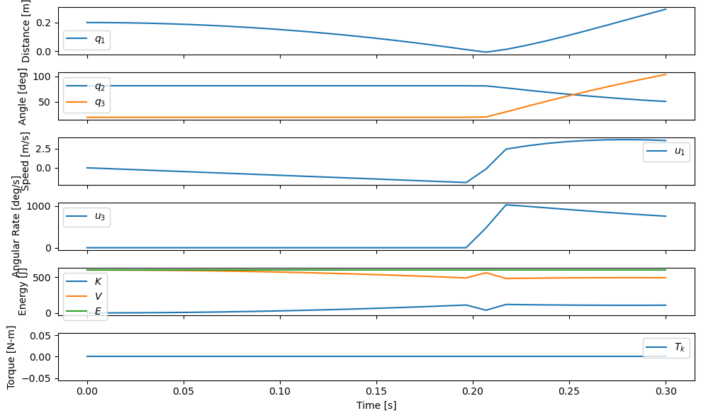
Now we get a bouncing jumper. This system should also still be conservative and we see that the energy stored in the foot spring is consumed from the loss of kinetic energy as the velocity goes to zero and that total energy is constant.

Nonconservative Simulation

Now we will give some damping to the Hunt-Crossely model by setting \(c_f=1\times10^5\).

p_vals = np.array([
  0.101,  # Ia,
  0.282,  # Ib,
  1e5,    # cf,
  0.0,    # ck,
  0.387,  # da,
  0.193,  # db,
  9.81,   # g,
  5e7,    # kf,
  0.0,    # kk,
  0.611,  # la,
  0.424,  # lb,
  6.769,  # ma,
  17.01,  # mb,
  3.0,    # mf,
  32.44,  # mu
])

t0, tf, fps = 0.0, 0.3, 100
ts_dae, xs_dae, Ks, Vs, Es, Tks = simulate(t0, tf, fps, x0, xd0, p_vals, eval_r)

HTML(animate_linkage(ts_dae, xs_dae, p_vals).to_jshtml(fps=fps))

Once Loop Reflect

plot_results(ts_dae, xs_dae, Ks, Vs, Es, Tks);

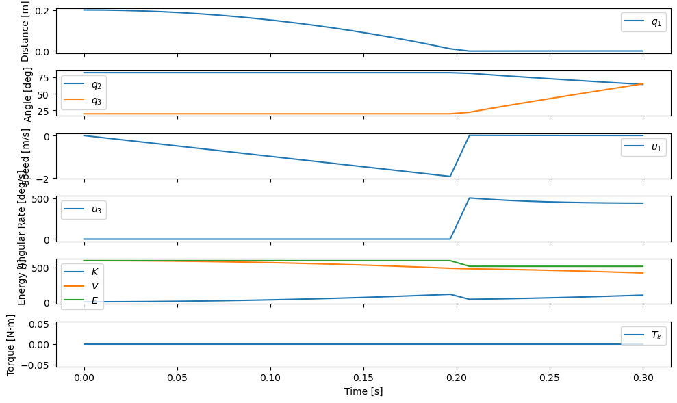
Now we see a clear energy dissipation from the system due to the foot-ground collision, i.e. the drop in \(E\).

Simulation with Passive Knee Torques

In this simulation, we include some passive stiffness and damping at the knee joint.

p_vals = np.array([
  0.101,  # Ia,
  0.282,  # Ib,
  1e5,    # cf,
  30.0,   # ck,
  0.387,  # da,
  0.193,  # db,
  9.81,   # g,
  5e7,    # kf,
  10.0,   # kk,
  0.611,  # la,
  0.424,  # lb,
  6.769,  # ma,
  17.01,  # mb,
  3.0,    # mf,
  32.44,  # mu
])

x0, xd0 = setup_initial_conditions(0.0, np.deg2rad(5.0), 0.0, 0.0)

t0, tf, fps = 0.0, 3.0, 60
ts_dae, xs_dae, Ks, Vs, Es, Tks = simulate(t0, tf, fps, x0, xd0, p_vals, eval_r)

HTML(animate_linkage(ts_dae, xs_dae, p_vals).to_jshtml(fps=fps))

Once Loop Reflect

plot_results(ts_dae, xs_dae, Ks, Vs, Es, Tks);

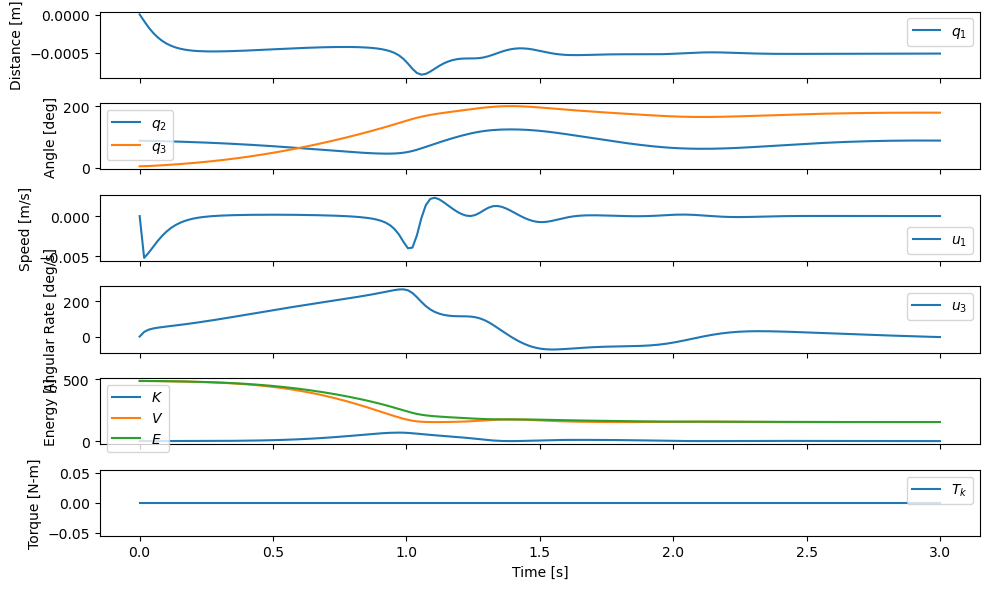
Notice that the knee collapses more slowly due to the damping and in the totarl energy plot the energy loss due to the non-conservative knee damping can be clearly seen.

Simulation with Active Knee Torques

Now that we likely have a reasonable passive model of a jumper we can try to make it jump by added energy to the system through the knee torque \(T_k\). We have a symbol for the specified time varying quantity and the simulation code has been designed above to accept a function that calculates \(T_k\) at any time instance. We’ll let the thigh fall and then give a constant torque to drive the thigh back up for a just two tenths of a second.

def eval_r(t, x, p):

    if t < 0.9:
        Tk = [0.0]
    elif t > 1.1:
        Tk = [0.0]
    else:
        Tk = [900.0]

    return Tk

p_vals = np.array([
  0.101,  # Ia,
  0.282,  # Ib,
  1e5,    # cf,
  30.0,   # ck,
  0.387,  # da,
  0.193,  # db,
  9.81,   # g,
  5e7,    # kf,
  10.0,   # kk,
  0.611,  # la,
  0.424,  # lb,
  6.769,  # ma,
  17.01,  # mb,
  3.0,    # mf,
  32.44,  # mu
])

We’ll start the simulation with the foot on the ground and with a slight knee bend.

x0, xd0 = setup_initial_conditions(0.0, np.deg2rad(5.0), 0.0, 0.0)

t0, tf, fps = 0.0, 2.0, 60
ts_dae, xs_dae, Ks, Vs, Es, Tks = simulate(t0, tf, fps, x0, xd0, p_vals, eval_r)

HTML(animate_linkage(ts_dae, xs_dae, p_vals).to_jshtml(fps=fps))

Once Loop Reflect

plot_results(ts_dae, xs_dae, Ks, Vs, Es, Tks);

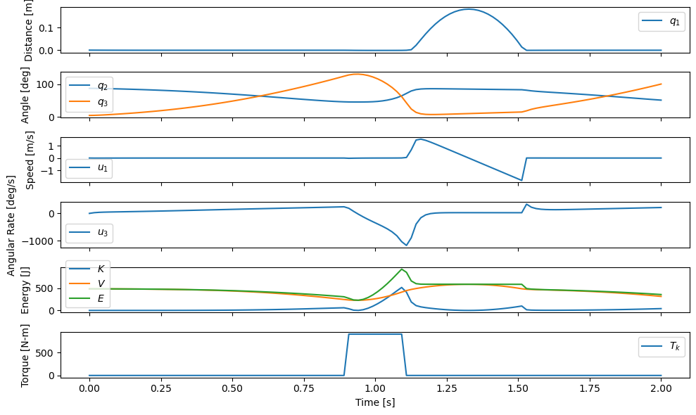
The final simulation works and gives a reasonably realistic looking jump. When examining the total energy \(E\) you can see how the applied knee torque adds energy to the system to cause the jump.