Vectors
Note
You can download this example as a Python script:
vectors.py or Jupyter Notebook:
vectors.ipynb.
import sympy as sm
import sympy.physics.mechanics as me
sm.init_printing(use_latex='mathjax')
class ReferenceFrame(me.ReferenceFrame):

    def __init__(self, *args, **kwargs):

        kwargs.pop('latexs', None)

        lab = args[0].lower()
        tex = r'\hat{{{}}}_{}'

        super(ReferenceFrame, self).__init__(*args,
                                             latexs=(tex.format(lab, 'x'),
                                                     tex.format(lab, 'y'),
                                                     tex.format(lab, 'z')),
                                             **kwargs)
me.ReferenceFrame = ReferenceFrame
Learning Objectives
After completing this chapter readers will be able to:
State the properties of a vectors.
Determine what scalars a vector is a function of.
Add, subtract, scale, negate, normalize vectors.
Dot and cross vectors with each other.
Express vectors in different reference frames.
Define vectors with components expressed in different reference frames.
Create position vectors between points using reference frame unit vectors.
What is a vector?
Vectors have three characteristics:
magnitude
orientation
sense
The direction the vector points is derived from both the orientation and the sense. Vectors are equal when all three characteristics are the same.

Fig. 10 Three characteristics of vectors: magnitude, orientation, and sense.
Note
In this text we will distinguish scalar variables, e.g. \(v\), from vectors by including a bar over the top of the symbol, e.g. \(\bar{v}\). Vectors will be drawn as follows:

Fig. 11 Various ways vectors will be drawn in figures.

Fig. 12 See right-hand rule for a refresher on right handed systems.
Right_hand_rule_simple.png: The original uploader was Schorschi2 at German Wikipedia.derivative work: Wizard191, Public domain, via Wikimedia Commons
Vectors have these mathematical properties:
scalar multiplicative: \(\bar{v} = \lambda\bar{u}\) where \(\lambda\) can only change the magnitude and the sense of the vector, i.e. \(\bar{v}\) and \(\bar{u}\) have the same orientation
commutative: \(\bar{u} + \bar{v} = \bar{v} + \bar{u}\)
distributive: \(\lambda(\bar{u} + \bar{v}) = \lambda\bar{u} + \lambda\bar{v}\)
associative: \((\bar{u} + \bar{v}) + \bar{w} = \bar{u} + (\bar{v} + \bar{w})\)
Unit vectors are vectors with a magnitude of \(1\). If the magnitude of \(\bar{v}\) is 1, then we indicate this with \(\hat{v}\). Any vector has an associated unit vector with the same orientation and sense, found by:
where \(|\bar{u}|\) is the Euclidean norm (2-norm), or magnitude, of the vector \(\bar{u}\).
Vector Functions
Vectors can be functions of scalar variables. If a change in scalar variable \(q\) changes the magnitude and/or direction of \(\bar{v}\) when observed from \(A\), \(\bar{v}\) is a vector function of \(q\) in \(A\). It is possible that \(\bar{v}\) may not be a vector function of scalar variable \(q\) when observed from another reference frame, i.e. the function dependency of a vector on a scalar depends on the reference frame it is observed from.
Let vector \(\bar{v}\) be a function of \(n\) scalars \(q_1,q_2,\ldots,q_n\) in \(A\). If we introduce \(\hat{a}_x,\hat{a}_y,\hat{a}_z\) as a set of mutually perpendicular unit vectors fixed in \(A\), then these unit vectors are constant when observed from \(A\). There are then three unique scalar functions \(v_x,v_y,v_z\) of \(q_1,q_2,\ldots,q_n\) such that:
\(v_x \hat{a}_x\) is called the \(\hat{a}_x\) component of \(\bar{v}\) and \(v_x\) is called measure number of \(\bar{v}\). Since the components are mutually perpendicular the measure number can also be found from the dot product of \(\bar{v}\) and the respective unit vector:
which is the projection of \(\bar{v}\) onto each unit vector. When written this way we can say that \(\bar{v}\) is expressed in \(A\). See sections 1.1-1.3 in [Kane1985] for a more general explanation.
Addition
When we add vector \(\bar{w}\) to vector \(\bar{v}\), the result is a vector that starts at the tail of \(\bar{v}\) and ends at the tip of \(\bar{w}\):

Fig. 13 Graphical vector addition
Vectors in SymPy Mechanics are created by first introducing a reference frame and using its associated unit vectors to construct vectors of arbitrary magnitude and direction.
N = me.ReferenceFrame('N')
Now introduce some scalar variables:
a, b, c, d, e, f = sm.symbols('a, b, c, d, e, f')
The simplest 3D non-unit vector is made up of a single component:
v = a*N.x
v
A, possible more familiar, column matrix form of a vector is accessed with the
to_matrix().
v.to_matrix(N)
Fully 3D and arbitrary vectors can be created by providing a measure number for each unit vector of \(N\):
w = a*N.x + b*N.y + c*N.z
w
And the associated column matrix form:
w.to_matrix(N)
Vector addition works by adding the measure numbers of each common component:
SymPy Mechanics vectors work as expected:
x = d*N.x + e*N.y + f*N.z
x
w + x
Scaling
Multiplying a vector by a scalar changes its magnitude, but not its orientation. Scaling by a negative number changes a vector’s magnitude and reverses its sense (rotates it by \(\pi\) radians).

Fig. 14 Vector scaling
y = 2*w
y
z = -w
z
Exercise
Create three vectors that lie in the \(xy\) plane of reference frame \(N\) where each vector is:
of length \(l\) that is at an angle of \(\frac{\pi}{4}\) degrees from the \(\hat{n}_x\) unit vector.
of length \(10\) and is in the \(-\hat{n}_y\) direction
of length \(l\) and is \(\theta\) radians from the \(\hat{n}_y\) unit vector.
Finally, add vectors from 1 and 2 and substract \(5\) times the third vector.
Hint: SymPy has fundamental constants and trigonometic functions, for
example sm.tan, sm.pi.
Solution
N = me.ReferenceFrame('N')
l, theta = sm.symbols('l, theta')
v1 = l*sm.cos(sm.pi/4)*N.x + l*sm.sin(sm.pi/4)*N.y
v1
v2 = -10*N.y
v2
v3 = -l*sm.sin(theta)*N.x + l*sm.cos(theta)*N.y
v3
v1 + v2 - 5*v3
Dot Product
The dot product, which yields a scalar quantity, is defined as:
where \(\theta\) is the angle between the two vectors. For arbitrary measure numbers this results in the following:

Fig. 15 Vector dot product
The dot product has these properties:
You can pull out scalars: \(c \bar{u} \cdot d \bar{v} = cd (\bar{u} \cdot \bar{v})\)
Order does not matter (commutative multiplication): \(\bar{u} \cdot \bar{v} = \bar{v} \cdot \bar{u}\)
You can distribute: \(\bar{u} \cdot (\bar{v} + \bar{w}) = \bar{u} \cdot \bar{v} + \bar{u} \cdot \bar{w}\)
The dot product is often used to determine:
the angle between two vectors: \(\theta = \arccos\frac{\bar{a} \cdot \bar{b}}{|\bar{a}|\bar{b}|}\)
a vector’s magnitude: \(|\bar{v}| = \sqrt{\bar{v} \cdot \bar{v}}\)
the length of a vector along a direction of another vector \(\hat{u}\) (called the projection): \(\mbox{proj}_{\hat{u}} \bar{v} = \bar{v} \cdot \hat{u}\)
if two vectors are perpendicular: \(\bar{v} \cdot \bar{w} = 0 \mbox{ if and only if }\bar{v} \perp \bar{w}\)
Compute power: \(P = \bar{F} \cdot \bar{v}\), where \(\bar{F}\) is a force vector and \(\bar{v}\) is the velocity of the point the force is acting on.
Also, dot products are used to convert a vector equation into a scalar equation by “dotting” an entire equation with a vector.
N = me.ReferenceFrame('N')
w = a*N.x + b*N.y + c*N.z
x = d*N.x + e*N.y + f*N.z
The dot() function
calculates the dot product:
me.dot(w, x)
The method form is equivalent:
w.dot(x)
You can compute a unit vector \(\hat{w}\) in the same direction as
\(\bar{w}\) with the
normalize() method:
w.normalize()
Exercise
Write your own function that normalizes an arbitrary vector and show that it
gives the same result as w.normalize().
Solution
def normalize(vector):
    return vector/sm.sqrt(me.dot(vector, vector))

normalize(w)
SymPy Mechanics vectors also have a method
magnitude() which is
helpful:
w.magnitude()
w/w.magnitude()
Exercise
Given the vectors \(\bar{v}_1 = a \hat{n}_x + b\hat{n}_y + a \hat{n}_z\) and \(\bar{v}_2=b \hat{n}_x + a\hat{n}_y + b \hat{n}_z\) find the angle between the two vectors using the dot product.
Solution
N = me.ReferenceFrame('N')
v1 = a*N.x + b*N.y + a*N.z
v2 = b*N.x + a*N.y + b*N.z
sm.acos(v1.dot(v2) / (v1.magnitude()*v2.magnitude()))
Cross Product
The cross product, which yields a vector quantity, is defined as:
where \(\theta\) is the angle between the two vectors, and \(\hat{u}\) is the unit vector perpendicular to both \(\bar{v}\) and \(\bar{w}\) whose sense is given by the right-hand rule. For arbitrary measure numbers this results in the following:

Fig. 16 Vector cross product
Some properties of cross products are:
Crossing a vector with itself “cancels” it: \(\bar{a} \times \bar{a} = \bar{0}\)
You can pull out scalars: \(c \bar{a} \times d \bar{b} = cd (\bar{a} \times \bar{b})\)
Order DOES matter (because of the right-hand rule): \(\bar{a} \times \bar{b} = -\bar{b} \times \bar{a}\)
You can distribute: \(\bar{a} \times (\bar{b} + \bar{c}) = \bar{a} \times \bar{b} + \bar{a} \times \bar{c}\)
They are NOT associative: \(\bar{a} \times (\bar{b} \times \bar{c}) \neq (\bar{a} \times \bar{b}) \times \bar{c}\)
The cross product is used to:
obtain a vector/direction perpendicular to two other vectors
determine if two vectors are parallel: \(\bar{v} \times \bar{w} = \bar{0} \mbox{ if } \bar{v} \parallel \bar{w}\)
compute moments: \(\bar{r} \times \bar{F}\)
compute the area of a triangle
SymPy Mechanics can calculate cross products with the
cross() function:
N = me.ReferenceFrame('N')
w = a*N.x + b*N.y + c*N.z
w
x = d*N.x + e*N.y + f*N.z
x
me.cross(w, x)
The method form is equivalent:
w.cross(x)
Exercise
Given three points located in reference frame \(N\) by:
Find the area of the triangle bounded by these three points using the cross product.
Hint: Search online for the relationship of the cross product to triangle area.
Solution
N = me.ReferenceFrame('N')

p1 = 23*N.x - 12* N.y
p2 = 16*N.x + 2*N.y - 4*N.z
p3 = N.x + 14*N.z

me.cross(p2 - p1, p3 - p1).magnitude() / 2
Vectors Expressed in Multiple Reference Frames
The notation of vectors represented by a scalar measure numbers associated with unit vectors becomes quite useful when you need to describe vectors with components in multiple reference frames. Utilizing unit vectors fixed in various frames is rather natural, with no need to think about direction cosine matrices.
N = me.ReferenceFrame('N')
A = me.ReferenceFrame('A')

a, b, theta = sm.symbols('a, b, theta')

v = a*A.x + b*N.y
v
All of the previously described operations work as expected:
v + v
If an orientation is established between the two reference frames, the
direction cosine transformations are handled for you and can be used to
naturally express the vector in either reference frame using the
express().
A.orient_axis(N, theta, N.z)

v.express(N)
v.express(A)
Relative Position Among Points
Take for example the balanced-arm lamp, which has multiple articulated joints configured in a way to balance the weight of the lamp in any configuration. Here are two examples:
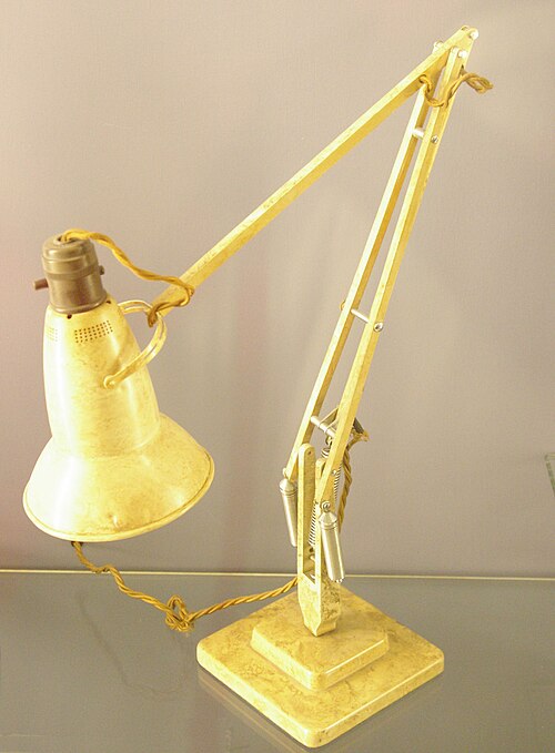
Fig. 17 Balanced-arm desk lamp.
Flickr user “renaissance chambara”, cropped by uploader, CC BY 2.0 https://creativecommons.org/licenses/by/2.0, via Wikimedia Commons
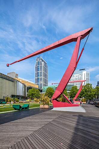
Fig. 18 Example of a huge balance-arm lamp in Rotterdam at the Schouwburgplein.
GraphyArchy, CC BY-SA 4.0 https://creativecommons.org/licenses/by-sa/4.0, via Wikimedia Commons
With those lamps in mind, Fig. 19 shows a diagram of a similar desk lamp with all necessary configuration information present. The base \(N\) is fixed to the desk. The first linkage \(A\) is oriented with respect to \(N\) by a \(z\textrm{-}x\) body fixed orientation through angles \(q_1\) and \(q_2\). Point \(P_1\) is fixed in \(N\) and is located at the center of the base. Linkage \(A\) is defined by points \(P_1\) and \(P_2\) which are separated by length \(l_1\) along the \(\hat{a}_z\) direction. Linkage \(B\) orients simply with respect to \(A\) about \(\hat{a}_x=\hat{b}_x\) through angle \(q_3\) and point \(P_3\) is \(l_2\) from \(P_2\) along \(\hat{b}_z\). Lastly, the lamp head \(C\) orients relative to \(B\) by a \(x\textrm{-}z\) body fixed orientation through angles \(q_4\) and \(q_5\). The center of the light bulb \(P_4\) is located relative to \(P_3\) by the distances \(l_3\) along \(\hat{c}_z\) and \(l_4\) along \(-\hat{c}_y\).

Fig. 19 Configuration diagram of a balanced-arm desk lamp.
We will use the following notation for vectors that indicate the relative position between two points:
which reads as the “position vector from \(P_1\) to \(P_2\)” or the “position vector of \(P_2\) with respect to \(P_1\)”. The tail of the vector is at \(P_1\) and the tip is at \(P_2\).
Exercise
Reread the Vector Functions section and answer the following questions:
Is \(\bar{r}^{P_2/P_1}\) vector function of \(q_1\) and \(q_2\) in N?
Is \(\bar{r}^{P_2/P_1}\) vector function of \(q_1\) and \(q_1\) in A?
Is \(\bar{r}^{P_2/P_1}\) vector function of \(q_3\) and \(q_4\) in N?
Is \(\bar{r}^{P_3/P_2}\) vector function of \(q_1\) and \(q_2\) in N?
Solution
See below how to use .free_symbols() to check your answers.
We can now write position vectors between pairs of points as we move from the base of the lamp to the light bulb. We’ll do so with SymPy Mechanics. First create the necessary symbols and reference frames.
q1, q2, q3, q4, q5 = sm.symbols('q1, q2, q3, q4, q5')
l1, l2, l3, l4 = sm.symbols('l1, l2, l3, l4')
N = me.ReferenceFrame('N')
A = me.ReferenceFrame('A')
B = me.ReferenceFrame('B')
C = me.ReferenceFrame('C')
Now establish the orientations, starting with \(A\)’s orientation relative to \(N\):
A.orient_body_fixed(N, (q1, q2, 0), 'ZXZ')
Note
Notice that the unneeded third simple orientation angle was set to zero.
Then \(B\)’s orientation relative to \(A\):
B.orient_axis(A, q3, A.x)
And finally \(C\)’s orientation relative to \(B\):
C.orient_body_fixed(B, (q4, q5, 0), 'XZX')
We can now create position vectors between pairs of points in the most convenient frame to do so, i.e. the reference frame in which both points lie on a line parallel to an existing unit vector. The intermediate vectors that connect \(P_1\) to \(P_2\), \(P_2\) to \(P_3\), and \(P_3\) to \(P_4\) are:
R_P1_P2 = l1*A.z
R_P2_P3 = l2*B.z
R_P3_P4 = l3*C.z - l4*C.y
The position vector from \(P_1\) to \(P_4\) is then found by vector addition:
R_P1_P4 = R_P1_P2 + R_P2_P3 + R_P3_P4
R_P1_P4
To convince you of the utility of our vector notation, have a look at what \(\bar{r}^{P_4/P_1}\) looks like if expressed completely in the \(N\) frame:
R_P1_P4.express(N)
If you have properly established your orientations and position vectors, SymPy Mechanics can help you determine the answers to the previous exercise. Expressing \(\bar{r}^{P2/P1}\) in \(N\) can show us which scalar variables that vector function depends on in \(N\).
R_P1_P2.express(N)
By inspection, we see the variables are \(l_1,q_1,q_2\). The
free_symbols() function
can extract these scalars directly:
R_P1_P2.free_symbols(N)
Warning
free_symbols() shows all SymPy Symbol objects, but will not show
Function() objects. In the next chapter we will introduce a way to do
the same thing when functions of time are present in your vector
expressions.
Similarly, other vector functions can be inspected:
R_P1_P2.free_symbols(A)
R_P1_P4.free_symbols(N)