Equations of Motion with Nonholonomic Constraints

Note

You can download this example as a Python script: nonholonomic-eom.py or Jupyter Notebook: nonholonomic-eom.ipynb.

from IPython.display import HTML
from matplotlib.animation import FuncAnimation
from scipy.integrate import solve_ivp
import matplotlib.pyplot as plt
import numpy as np
import sympy as sm
import sympy.physics.mechanics as me

me.init_vprinting(use_latex='mathjax')

class ReferenceFrame(me.ReferenceFrame):

    def __init__(self, *args, **kwargs):

        kwargs.pop('latexs', None)

        lab = args[0].lower()
        tex = r'\hat{{{}}}_{}'

        super(ReferenceFrame, self).__init__(*args,
                                             latexs=(tex.format(lab, 'x'),
                                                     tex.format(lab, 'y'),
                                                     tex.format(lab, 'z')),
                                             **kwargs)
me.ReferenceFrame = ReferenceFrame

Learning Objectives

After completing this chapter readers will be able to:

• formulate the \(p\) dynamical differential equations for a nonholonomic system

• simulate a nonholonomic multibody system

• calculate trajectories of dependent speeds

Introduction

In chapters, Holonomic Constraints and Nonholonomic Constraints, I introduced two types of constraints: holonomic (configuration) constraints and nonholonomic (motion) constraints. Holonomic constraints are nonlinear constraints in the coordinates [1]. Nonholonomic constraints are linear in the generalized speeds, by definition. We will address the nonholonomic equations of motion first, as they are slightly easier to deal with.

[1]

They can be linear in the coordinates, but then there is little reason not to solve for the depedendent coordinates and eliminate them.

Nonholonomic constraint equations are linear in both the independent and dependent generalized speeds (see Sec. Snakeboard). We have shown that you can explicitly solve for the dependent generalized speeds \(\bar{u}_r\) as a function of the independent generalized speeds \(\bar{u}_s\). This means that number of dynamical differential equations can be reduced to \(p\) from \(n\) with \(m\) nonholonomic constraints. Recall that the nonholonomic constraints take this form:

(201)\[\bar{f}_n(\bar{u}_s, \bar{u}_r, \bar{q}, t) = \mathbf{M}_n\bar{u}_r + \bar{g}_n = 0 \in \mathbb{R}^m\]

and \(u_r\) can be solved for as so:

(202)\[\bar{u}_r = -\mathbf{M}_n(\bar{q}, t)^{-1}\bar{g}_n(\bar{u}_s, \bar{q}, t)\]

which is the same as Eq. (122) we originally developed:

(203)\[\begin{split}\bar{u}_r = \mathbf{A}_n \bar{u}_s + \bar{b}_n\\\end{split}\]

Using Eq. (202) equation we can now write our equations of motion as \(n\) kinematical differential equations and \(p\) dynamical differential equations.

(204)\[\begin{split}\bar{f}_k(\bar{u}_s, \dot{\bar{q}}, \bar{q}, t) = \mathbf{M}_k\dot{\bar{q}} + \bar{g}_k = 0 \in \mathbb{R}^n \\ \bar{f}_d(\dot{\bar{u}}_s, \bar{u}_s, \bar{q}, t) = \mathbf{M}_d\dot{\bar{u}}_s + \bar{g}_d = 0 \in \mathbb{R}^p\end{split}\]

and these can be written in explicit form:

(205)\[\begin{split}\dot{\bar{q}} = -\mathbf{M}_k(\bar{q}, t)^{-1} \bar{g}_k(\bar{u}_s, \bar{q}, t) \\ \dot{\bar{u}}_s = -\mathbf{M}_d(\bar{q}, t)^{-1} \bar{g}_d(\bar{u}_s, \bar{q}, t) \\\end{split}\]

This leaves us with \(n+p\) equations of motion, instead of \(2n\) equations seen in a holonomic system. Nonholonomic constraints reduce the number of degrees of freedom and thus fewer dynamical differential equations are necessary to fully describe the motion.

Snakeboard Equations of Motion

Let’s revisit the snakeboard example (see Sec. Snakeboard) and develop the equations of motion for that nonholonomic system. This system only has nonholonomic constraints and we selected \(u_1\) and \(u_2\) as the dependent speeds. For simplicity, we will assume that the mass and moments of inertia of the three bodies are the same.

Fig. 48 Configuration diagram of a planar Snakeboard model.

1. Declare all the variables

First introduce the necessary variables; adding \(I\) for the central moment of inertia of each body and \(m\) as the mass of each body. Then create column matrices for the various sets of variables.

q1, q2, q3, q4, q5 = me.dynamicsymbols('q1, q2, q3, q4, q5')
u1, u2, u3, u4, u5 = me.dynamicsymbols('u1, u2, u3, u4, u5')
l, I, m = sm.symbols('l, I, m')
t = me.dynamicsymbols._t

p = sm.Matrix([l, I, m])
q = sm.Matrix([q1, q2, q3, q4, q5])
us = sm.Matrix([u3, u4, u5])
ur = sm.Matrix([u1, u2])
u = ur.col_join(us)

q, ur, us, u, p

\[\begin{split}\displaystyle \left( \left[\begin{matrix}q_{1}\\q_{2}\\q_{3}\\q_{4}\\q_{5}\end{matrix}\right], \ \left[\begin{matrix}u_{1}\\u_{2}\end{matrix}\right], \ \left[\begin{matrix}u_{3}\\u_{4}\\u_{5}\end{matrix}\right], \ \left[\begin{matrix}u_{1}\\u_{2}\\u_{3}\\u_{4}\\u_{5}\end{matrix}\right], \ \left[\begin{matrix}l\\I\\m\end{matrix}\right]\right)\end{split}\]

We will also need column matrices for the time derivatives of each set of variables and some dictionaries to zero out any of these variables in various expressions we create.

qd = q.diff()
urd = ur.diff(t)
usd = us.diff(t)
ud = u.diff(t)

qd, urd, usd, ud

\[\begin{split}\displaystyle \left( \left[\begin{matrix}\dot{q}_{1}\\\dot{q}_{2}\\\dot{q}_{3}\\\dot{q}_{4}\\\dot{q}_{5}\end{matrix}\right], \ \left[\begin{matrix}\dot{u}_{1}\\\dot{u}_{2}\end{matrix}\right], \ \left[\begin{matrix}\dot{u}_{3}\\\dot{u}_{4}\\\dot{u}_{5}\end{matrix}\right], \ \left[\begin{matrix}\dot{u}_{1}\\\dot{u}_{2}\\\dot{u}_{3}\\\dot{u}_{4}\\\dot{u}_{5}\end{matrix}\right]\right)\end{split}\]

qd_zero = {qdi: 0 for qdi in qd}
ur_zero = {ui: 0 for ui in ur}
us_zero = {ui: 0 for ui in us}
urd_zero = {udi: 0 for udi in urd}
usd_zero = {udi: 0 for udi in usd}

qd_zero, ur_zero, us_zero

\[\displaystyle \left( \left\{ \dot{q}_{1} : 0, \ \dot{q}_{2} : 0, \ \dot{q}_{3} : 0, \ \dot{q}_{4} : 0, \ \dot{q}_{5} : 0\right\}, \ \left\{ u_{1} : 0, \ u_{2} : 0\right\}, \ \left\{ u_{3} : 0, \ u_{4} : 0, \ u_{5} : 0\right\}\right)\]

urd_zero, usd_zero

\[\displaystyle \left( \left\{ \dot{u}_{1} : 0, \ \dot{u}_{2} : 0\right\}, \ \left\{ \dot{u}_{3} : 0, \ \dot{u}_{4} : 0, \ \dot{u}_{5} : 0\right\}\right)\]

2. Establish the kinematics

The following code sets up the orientations, positions, and velocities exactly as done in the original example. All of the velocities are in terms of \(\bar{q}\) and \(\dot{\bar{q}}\).

N = me.ReferenceFrame('N')
A = me.ReferenceFrame('A')
B = me.ReferenceFrame('B')
C = me.ReferenceFrame('C')

A.orient_axis(N, q3, N.z)
B.orient_axis(A, q4, A.z)
C.orient_axis(A, q5, A.z)

A.ang_vel_in(N)
B.ang_vel_in(N)
C.ang_vel_in(N)

O = me.Point('O')
Ao = me.Point('A_o')
Bo = me.Point('B_o')
Co = me.Point('C_o')

Ao.set_pos(O, q1*N.x + q2*N.y)
Bo.set_pos(Ao, l/2*A.x)
Co.set_pos(Ao, -l/2*A.x)

O.set_vel(N, 0)
Bo.v2pt_theory(Ao, N, A)
Co.v2pt_theory(Ao, N, A);

3. Specify the kinematical differential equations

Now create the \(n=5\) kinematical differential equations \(\bar{f}_k\):

fk = sm.Matrix([
    u1 - q1.diff(t),
    u2 - q2.diff(t),
    u3 - l*q3.diff(t)/2,
    u4 - q4.diff(t),
    u5 - q5.diff(t),
])

It is a good idea to use find_dynamicsymbols() to check which functions of time are present in the various equations. This function is invaluable when the equations begin to become very large.

me.find_dynamicsymbols(fk)

\[\displaystyle \left\{q_{1}, q_{2}, q_{3}, q_{4}, q_{5}, u_{1}, u_{2}, u_{3}, u_{4}, u_{5}, \dot{q}_{1}, \dot{q}_{2}, \dot{q}_{3}, \dot{q}_{4}, \dot{q}_{5}\right\}\]

Symbolically solve these equations for \(\dot{\bar{q}}\) and setup a dictionary we can use for substitutions:

Mk = fk.jacobian(qd)
gk = fk.xreplace(qd_zero)
qd_sol = -Mk.LUsolve(gk)
qd_repl = dict(zip(qd, qd_sol))
qd_repl

\[\displaystyle \left\{ \dot{q}_{1} : u_{1}, \ \dot{q}_{2} : u_{2}, \ \dot{q}_{3} : \frac{2 u_{3}}{l}, \ \dot{q}_{4} : u_{4}, \ \dot{q}_{5} : u_{5}\right\}\]

4. Establish the nonholonomic constraints

Create the \(m=2\) nonholonomic constraints:

fn = sm.Matrix([Bo.vel(N).dot(B.y), Co.vel(N).dot(C.y)])
fn

\[\begin{split}\displaystyle \left[\begin{matrix}\frac{l \cos{\left(q_{4} \right)} \dot{q}_{3}}{2} + \left(- \sin{\left(q_{3} \right)} \sin{\left(q_{4} \right)} + \cos{\left(q_{3} \right)} \cos{\left(q_{4} \right)}\right) \dot{q}_{2} + \left(- \sin{\left(q_{3} \right)} \cos{\left(q_{4} \right)} - \sin{\left(q_{4} \right)} \cos{\left(q_{3} \right)}\right) \dot{q}_{1}\\- \frac{l \cos{\left(q_{5} \right)} \dot{q}_{3}}{2} + \left(- \sin{\left(q_{3} \right)} \sin{\left(q_{5} \right)} + \cos{\left(q_{3} \right)} \cos{\left(q_{5} \right)}\right) \dot{q}_{2} + \left(- \sin{\left(q_{3} \right)} \cos{\left(q_{5} \right)} - \sin{\left(q_{5} \right)} \cos{\left(q_{3} \right)}\right) \dot{q}_{1}\end{matrix}\right]\end{split}\]

and rewrite them in terms of the generalized speeds:

fn = fn.xreplace(qd_repl)
fn

\[\begin{split}\displaystyle \left[\begin{matrix}\left(- \sin{\left(q_{3} \right)} \sin{\left(q_{4} \right)} + \cos{\left(q_{3} \right)} \cos{\left(q_{4} \right)}\right) u_{2} + \left(- \sin{\left(q_{3} \right)} \cos{\left(q_{4} \right)} - \sin{\left(q_{4} \right)} \cos{\left(q_{3} \right)}\right) u_{1} + u_{3} \cos{\left(q_{4} \right)}\\\left(- \sin{\left(q_{3} \right)} \sin{\left(q_{5} \right)} + \cos{\left(q_{3} \right)} \cos{\left(q_{5} \right)}\right) u_{2} + \left(- \sin{\left(q_{3} \right)} \cos{\left(q_{5} \right)} - \sin{\left(q_{5} \right)} \cos{\left(q_{3} \right)}\right) u_{1} - u_{3} \cos{\left(q_{5} \right)}\end{matrix}\right]\end{split}\]

me.find_dynamicsymbols(fn)

\[\displaystyle \left\{q_{3}, q_{4}, q_{5}, u_{1}, u_{2}, u_{3}\right\}\]

With the nonholonomic constraint equations we choose \(\bar{u}_r=[u_1 \ u_2]^T\) and symbolically for these dependent speeds.

Mn = fn.jacobian(ur)
gn = fn.xreplace(ur_zero)
ur_sol = Mn.LUsolve(-gn)
ur_repl = dict(zip(ur, ur_sol))

In our case, the dependent generalized speeds are only a function of one independent generalized speed, \(u_3\).

me.find_dynamicsymbols(ur_sol)

\[\displaystyle \left\{q_{3}, q_{4}, q_{5}, u_{3}\right\}\]

Exercise

Why does \(u_1\) and \(u_2\) not depend on \(q_1,q_2,u_4\) and \(u_5\)?

Our kinematical differential equations can now be rewritten in terms of the independent generalized speeds. We only need to rewrite \(\bar{g}_k\) for later use in our numerical functions.

gk = gk.xreplace(ur_repl)

me.find_dynamicsymbols(gk)

\[\displaystyle \left\{q_{3}, q_{4}, q_{5}, u_{3}, u_{4}, u_{5}\right\}\]

5. Rewrite velocities in terms of independent speeds

The snakeboard model, as described, has no generalized active forces because there are no contributing external forces acting on the system, so we only need to generate the nonholonomic generalized inertia forces \(\tilde{F}_r^*\). We now then calculate the velocities we will need to form \(\tilde{F}_r^*\) and make sure they are written only in terms of the independent generalized speeds.

N_w_A = A.ang_vel_in(N).xreplace(qd_repl).xreplace(ur_repl)
N_w_B = B.ang_vel_in(N).xreplace(qd_repl).xreplace(ur_repl)
N_w_C = C.ang_vel_in(N).xreplace(qd_repl).xreplace(ur_repl)
N_v_Ao = Ao.vel(N).xreplace(qd_repl).xreplace(ur_repl)
N_v_Bo = Bo.vel(N).xreplace(qd_repl).xreplace(ur_repl)
N_v_Co = Co.vel(N).xreplace(qd_repl).xreplace(ur_repl)

vels = (N_w_A, N_w_B, N_w_C, N_v_Ao, N_v_Bo, N_v_Co)

for vel in vels:
    print(me.find_dynamicsymbols(vel, reference_frame=N))

{u3(t)}
{u4(t), u3(t)}
{u5(t), u3(t)}
{q5(t), q3(t), q4(t), u3(t)}
{q5(t), q3(t), q4(t), u3(t)}
{q5(t), q3(t), q4(t), u3(t)}

6. Compute the partial velocities

With the velocities only in terms of the independent generalized speeds, we can calculate the \(p\) nonholonomic partial velocities:

w_A, w_B, w_C, v_Ao, v_Bo, v_Co = me.partial_velocity(vels, us, N)

7. Rewrite the accelerations in terms of the independent generalized speeds

We can also write the accelerations in terms of only the independent generalized speeds, their time derivatives, and the generalized coordinates. To do so, we need to differentiate the nonholonomic constraints so that we can eliminate the dependent generalized accelerations, \(\dot{\bar{u}}_r\). Differentiating the constraints with respect to time and then substituting for the dependent generalized speeds gives us equations for the dependent generalized accelerations.

(206)\[\begin{split}\dot{\bar{f}}_n(\dot{\bar{u}}_r, \dot{\bar{u}}_s, \bar{u}_s, \bar{u}_r, \bar{q}, t) = \mathbf{M}_{nd}\dot{\bar{u}}_r + \bar{g}_{nd}= 0 \in \mathbb{R}^m\\ \dot{\bar{u}}_r = -\mathbf{M}_{nd}(\bar{q}, t)^{-1} \bar{g}_{nd}(\dot{\bar{u}}_s, \bar{u}_s, \bar{q}, t)\end{split}\]

First, time differentiate the nonholonomic constraints and eliminate the time derivatives of the generalized coordinates.

fnd = fn.diff(t).xreplace(qd_repl)

me.find_dynamicsymbols(fnd)

\[\displaystyle \left\{q_{3}, q_{4}, q_{5}, u_{1}, u_{2}, u_{3}, u_{4}, u_{5}, \dot{u}_{1}, \dot{u}_{2}, \dot{u}_{3}\right\}\]

Now solve for the dependent generalized accelerations. Note that I replace the dependent generalized speeds in \(\bar{g}_{nd}\) instead of \(\dot{\bar{f}}_n\) earlier. This is to avoid replacing the u_1 and u_2 terms in the Derivative(u1, t) and Derivative(u2, t) terms.

Mnd = fnd.jacobian(urd)
gnd = fnd.xreplace(urd_zero).xreplace(ur_repl)
urd_sol = Mnd.LUsolve(-gnd)
urd_repl = dict(zip(urd, urd_sol))

me.find_dynamicsymbols(urd_sol)

\[\displaystyle \left\{q_{3}, q_{4}, q_{5}, u_{3}, u_{4}, u_{5}, \dot{u}_{3}\right\}\]

8. Create the generalized forces

Now we can form the inertia forces and inertia torques. First check what derivatives appear in the accelerations.

Rs_Ao = -m*Ao.acc(N)
Rs_Bo = -m*Bo.acc(N)
Rs_Co = -m*Co.acc(N)

(me.find_dynamicsymbols(Rs_Ao, reference_frame=N) |
 me.find_dynamicsymbols(Rs_Bo, reference_frame=N) |
 me.find_dynamicsymbols(Rs_Co, reference_frame=N))

\[\displaystyle \left\{q_{1}, q_{2}, q_{3}, \ddot{q}_{1}, \ddot{q}_{2}, \dot{q}_{3}, \ddot{q}_{3}\right\}\]

We’ll need to replace the \(\ddot{\bar{q}}\) first and then the \(\dot{\bar{q}}\). Create the first replacement by differentiating the expressions for \(\dot{\bar{q}}\).

Warning

If you use chained replacements, e.g. .xreplace().xreplace().xreplace() you have to be careful about the order of replacements so that you don’t substitute symbols inside a derivative, e.g. Derivative(u, t). If you have expr = Derivative(u, t) + u then you need to replace the entire derivative first: expr.xreplace({u.diff(): 1}).xreplace({u: 2}).

qdd_repl = {k.diff(t): v.diff(t).xreplace(urd_repl) for k, v in qd_repl.items()}

Rs_Ao = -m*Ao.acc(N).xreplace(qdd_repl).xreplace(qd_repl)
Rs_Bo = -m*Bo.acc(N).xreplace(qdd_repl).xreplace(qd_repl)
Rs_Co = -m*Co.acc(N).xreplace(qdd_repl).xreplace(qd_repl)

(me.find_dynamicsymbols(Rs_Ao, reference_frame=N) |
 me.find_dynamicsymbols(Rs_Bo, reference_frame=N) |
 me.find_dynamicsymbols(Rs_Co, reference_frame=N))

\[\displaystyle \left\{q_{3}, q_{4}, q_{5}, u_{3}, u_{4}, u_{5}, \dot{u}_{3}\right\}\]

The motion is planar so the generalized inertia torques are simply angular accelerations dotted with the central inertia dyadics.

I_A_Ao = I*me.outer(A.z, A.z)
I_B_Bo = I*me.outer(B.z, B.z)
I_C_Co = I*me.outer(C.z, C.z)

Now have a look at which functions are present in the inertia torques:

Ts_A = -A.ang_acc_in(N).dot(I_A_Ao)
Ts_B = -B.ang_acc_in(N).dot(I_B_Bo)
Ts_C = -C.ang_acc_in(N).dot(I_C_Co)

(me.find_dynamicsymbols(Ts_A, reference_frame=N) |
 me.find_dynamicsymbols(Ts_B, reference_frame=N) |
 me.find_dynamicsymbols(Ts_C, reference_frame=N))

\[\displaystyle \left\{q_{3}, q_{4}, q_{5}, \ddot{q}_{3}, \ddot{q}_{4}, \ddot{q}_{5}\right\}\]

and eliminate the dependent generalized accelerations:

Ts_A = -A.ang_acc_in(N).dot(I_A_Ao).xreplace(qdd_repl)
Ts_B = -B.ang_acc_in(N).dot(I_B_Bo).xreplace(qdd_repl)
Ts_C = -C.ang_acc_in(N).dot(I_C_Co).xreplace(qdd_repl)

(me.find_dynamicsymbols(Ts_A, reference_frame=N) |
 me.find_dynamicsymbols(Ts_B, reference_frame=N) |
 me.find_dynamicsymbols(Ts_C, reference_frame=N))

\[\displaystyle \left\{u_{3}, u_{4}, u_{5}, \dot{u}_{3}, \dot{u}_{4}, \dot{u}_{5}\right\}\]

9. Formulate the dynamical differential equations

All of the components are present to formulate the nonholonomic generalized inertia forces. After we form them, make sure they are only a function of the independent generalized speeds, their time derivatives, and the generalized coordinates.

Frs = []
for i in range(len(us)):
    Frs.append(v_Ao[i].dot(Rs_Ao) + v_Bo[i].dot(Rs_Bo) + v_Co[i].dot(Rs_Co) +
               w_A[i].dot(Ts_A) + w_B[i].dot(Ts_B) + w_C[i].dot(Ts_C))
Frs = sm.Matrix(Frs)

me.find_dynamicsymbols(Frs)

\[\displaystyle \left\{q_{3}, q_{4}, q_{5}, u_{3}, u_{4}, u_{5}, \dot{u}_{3}, \dot{u}_{4}, \dot{u}_{5}\right\}\]

At this point you may have noticed that \(q_1\) and \(q_2\) have not appeared in any equations. This means that the dynamics do not depend on the planar location of the snakeboard. \(q_1\) and \(q_2\) are called ignorable coordinates if they do not appear in the equations of motion. It is only coincidence that the time derivatives of these ignorable coordinates are equal to the to dependent generalized speeds.

Lastly, extract the linear coefficients and the remainder for the dynamical differential equations.

Md = Frs.jacobian(usd)
gd = Frs.xreplace(usd_zero)

And one last time, check that \(\mathbf{M}_d\) and \(\mathbf{g}_d\) are only functions of the independent generalized speeds and the generalized coordinates.

me.find_dynamicsymbols(Md)

\[\displaystyle \left\{q_{3}, q_{4}, q_{5}\right\}\]

me.find_dynamicsymbols(gd)

\[\displaystyle \left\{q_{3}, q_{4}, q_{5}, u_{3}, u_{4}, u_{5}\right\}\]

We now have \(\mathbf{M}_k, \bar{g}_k, \mathbf{M}_d\) and \(\bar{g}_d\) and can proceed to numerical evaluation.

Simulate the Snakeboard

We now move to numerical evaluation for the simulation. First, create a function that evaluates the matrices of the equations of motion.

eval_kd = sm.lambdify((q, us, p), (Mk, gk, Md, gd), cse=True)

Now create a function that evaluates the right hand side of the explicit ordinary differential equations for use with solve_ivp().

def eval_rhs(t, x, p):
    """Returns the time derivative of the states.

    Parameters
    ==========
    t : float
    x : array_like, shape(8,)
       x = [q1, q2, q3, q4, q5, u3, u4, u5]
    p : array_like, shape(3,)
       p = [l, I, m]

    Returns
    =======
    xd : ndarray, shape(8,)
       xd = [q1d, q2d, q3d, q4d, q5d, u3d, u4d, u5d]

    """
    q, us = x[:5], x[5:]

    Mk, gk, Md, gd = eval_kd(q, us, p)

    qd = -np.linalg.solve(Mk, gk.squeeze())
    usd = -np.linalg.solve(Md, gd.squeeze())

    return np.hstack((qd, usd))

Now introduce some numeric values for the constant parameters and the initial condition of the state. I’ve selected some values here that will put the snakeboard in an initial state of motion.

p_vals = np.array([
    0.7,  # l [m]
    0.1,  # I [kg*m^2]
    1.0,  # m [kg]
])

q0 = np.array([
    0.0,  # q1 [m]
    0.0,  # q2 [m]
    0.0,  # q3 [rad]
    np.deg2rad(5.0),  # q4 [rad]
    -np.deg2rad(5.0),  # q5 [rad]
])

us0 = np.array([
    0.1,  # u3 [m/s]
    0.01,  # u4 [rad/s]
    -0.01,  # u5 [rad/s]
])

x0 = np.hstack((q0, us0))
p_vals, x0

(array([0.7, 0.1, 1. ]),
 array([ 0.        ,  0.        ,  0.        ,  0.08726646, -0.08726646,
         0.1       ,  0.01      , -0.01      ]))

Check whether eval_rhs() works with these arrays:

eval_rhs(1.0, x0, p_vals)

array([ 1.14300523,  0.        ,  0.28571429,  0.01      , -0.01      ,
        0.01143537, -0.03267249, -0.03267249])

We can now integrate the equations of motion to find the state trajectories. I setup the time array for the solution to correspond to 30 frames per second for later use in the animation of the motion.

t0, tf = 0.0, 8.0

fps = 20
ts = np.linspace(t0, tf, num=int(fps*(tf - t0)))

sol = solve_ivp(eval_rhs, (t0, tf), x0, args=(p_vals,), t_eval=ts)

xs = np.transpose(sol.y)

Now we can plot the state trajectories to see if there is realistic motion.

fig, axes = plt.subplots(2, 1, sharex=True)
fig.set_figwidth(10.0)

axes[0].plot(ts, xs[:, :2])
axes[0].legend(('$q_1$', '$q_2$'))
axes[0].set_ylabel('Distance [m]')

axes[1].plot(ts, np.rad2deg(xs[:, 2:5]))
axes[1].legend(('$q_3$', '$q_4$', '$q_5$'))
axes[1].set_ylabel('Angle [deg]')
axes[1].set_xlabel('Time [s]');

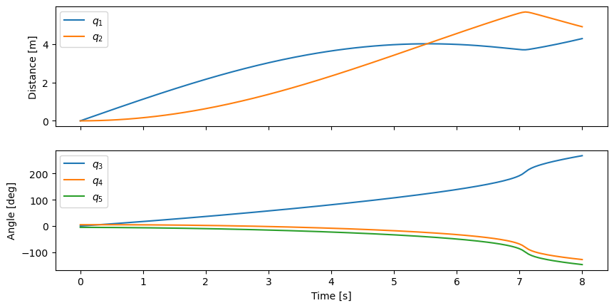
We see that the \(x\) and \(y\) positions vary over several meters and that there is a sharp transition around about 7 seconds. \(q_3(t)\) shows that the primary angle of the snakeboard grows with time and does almost a full rotation. Plotting the path on the ground plane of \(A_o\) gives a bit more insight to the motion.

fig, ax = plt.subplots()
fig.set_figwidth(10.0)

ax.plot(xs[:, 0], xs[:, 1])
ax.set_aspect('equal')
ax.set_xlabel('$q_1$ [m]')
ax.set_ylabel('$q_2$ [m]');

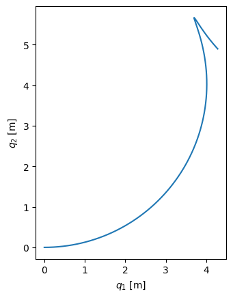
We see that the snakeboard curves to the left but eventually makes a very sharp trajectory change. An animation will provide an even more clear idea of the motion of this nonholonomic system.

Animate the Snakeboard

We will animate the snakeboard as a collection of lines and points and animate the 2D motion with matplotlib. First, create some new points that represent the location of the left and right wheels on bodies \(B\) and \(C\).

Bl = me.Point('B_l')
Br = me.Point('B_r')
Cr = me.Point('C_r')
Cl = me.Point('C_l')

Bl.set_pos(Bo, -l/4*B.y)
Br.set_pos(Bo, l/4*B.y)
Cl.set_pos(Co, -l/4*C.y)
Cr.set_pos(Co, l/4*C.y)

Create a function that numerically evaluates the Cartesian coordinates of all the points we want to plot given the generalized coordinates.

coordinates = Cl.pos_from(O).to_matrix(N)
for point in [Co, Cr, Co, Ao, Bo, Bl, Br]:
    coordinates = coordinates.row_join(point.pos_from(O).to_matrix(N))

eval_point_coords = sm.lambdify((q, p), coordinates, cse=True)
eval_point_coords(q0, p_vals)

array([[-0.36525225, -0.35      , -0.33474775, -0.35      ,  0.        ,
         0.35      ,  0.36525225,  0.33474775],
       [-0.17433407, -0.        ,  0.17433407, -0.        ,  0.        ,
         0.        , -0.17433407,  0.17433407],
       [ 0.        ,  0.        ,  0.        ,  0.        ,  0.        ,
         0.        ,  0.        ,  0.        ]])

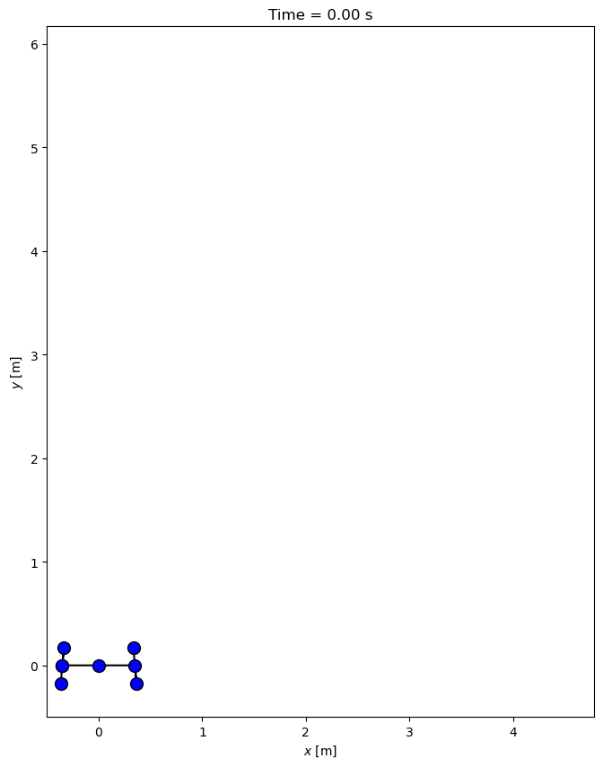
Now create a plot of the initial configuration:

x, y, z = eval_point_coords(q0, p_vals)

fig, ax = plt.subplots()
fig.set_size_inches((10.0, 10.0))
ax.set_aspect('equal')

lines, = ax.plot(x, y, color='black',
                 marker='o', markerfacecolor='blue', markersize=10)
# some empty lines to use for the wheel paths
bl_path, = ax.plot([], [])
br_path, = ax.plot([], [])
cl_path, = ax.plot([], [])
cr_path, = ax.plot([], [])

title_template = 'Time = {:1.2f} s'
title_text = ax.set_title(title_template.format(t0))
ax.set_xlim((np.min(xs[:, 0]) - 0.5, np.max(xs[:, 0]) + 0.5))
ax.set_ylim((np.min(xs[:, 1]) - 0.5, np.max(xs[:, 1]) + 0.5))
ax.set_xlabel('$x$ [m]')
ax.set_ylabel('$y$ [m]');

And, finally, animate the motion:

coords = []
for xi in xs:
     coords.append(eval_point_coords(xi[:5], p_vals))
coords = np.array(coords)  # shape(600, 3, 8)

def animate(i):
    title_text.set_text(title_template.format(sol.t[i]))
    lines.set_data(coords[i, 0, :], coords[i, 1, :])
    cl_path.set_data(coords[:i, 0, 0], coords[:i, 1, 0])
    cr_path.set_data(coords[:i, 0, 2], coords[:i, 1, 2])
    bl_path.set_data(coords[:i, 0, 6], coords[:i, 1, 6])
    br_path.set_data(coords[:i, 0, 7], coords[:i, 1, 7])

ani = FuncAnimation(fig, animate, len(sol.t))

HTML(ani.to_jshtml(fps=fps))

Once Loop Reflect

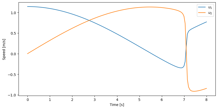
Calculating Dependent Speeds

Since we have eliminated the dependent generalized speeds (\(u_1\) and \(u_2\)) from the equations of motion, these are not computed from solve_ivp(). If these are needed, it is possible to calculate them using the constraint equations. Here I loop through time to calculate \(\bar{u}_r\) at each time step and then plot the results.

x = sm.Matrix([q1, q2, q3, q4, q5, u3, u4, u5])
eval_ur = sm.lambdify((x, p), ur_sol, cse=True)

ur_vals = []
for xi in xs:
    ur_vals.append(eval_ur(xi, p_vals))
ur_vals = np.array(ur_vals).squeeze()

fig, ax = plt.subplots()
fig.set_figwidth(10.0)
ax.plot(ts, ur_vals)
ax.set_ylabel('Speed [m/s]')
ax.set_xlabel('Time [s]')
ax.legend(['$u_1$', '$u_2$']);