Simulation and Visualization
Note
You can download this example as a Python script:
simulation.py or Jupyter Notebook:
simulation.ipynb.
import sympy as sm
import sympy.physics.mechanics as me
me.init_vprinting(use_latex='mathjax')
class ReferenceFrame(me.ReferenceFrame):
def __init__(self, *args, **kwargs):
kwargs.pop('latexs', None)
lab = args[0].lower()
tex = r'\hat{{{}}}_{}'
super(ReferenceFrame, self).__init__(*args,
latexs=(tex.format(lab, 'x'),
tex.format(lab, 'y'),
tex.format(lab, 'z')),
**kwargs)
me.ReferenceFrame = ReferenceFrame
Learning Objectives
After completing this chapter readers will be able to:
evaluate equations of motion numerically
numerically integrate the ordinary differential equations of a multibody system
plot the system’s state trajectories versus time
compare integration methods to observe integration error
create a simple animation of the motion of the multibody system
Numerical Integration
As mentioned at the end of the prior chapter, we will need to numerically integrate the equations of motion. If they are in explicit form, this integral describes how we can arrive at trajectories in time for the state variables by integrating with respect to time from an initial time \(t_0\) to a final time \(t_f\). Recall that the time derivative of the state \(\bar{x}\) is:
We can then find \(\bar{x}\) by integration with respect to time:
It is possible to form \(-\mathbf{M}_m^{-1}\bar{g}_m\) symbolically and it may be suitable or preferable for a given problem, but there are some possible drawbacks. For example, if the degrees of freedom are quite large, the resulting symbolic equations become exponentially more complex. Thus, it is generally best to move from symbolics to numerics before formulating the explicit ordinary differential equations.
Numerical Evaluation
The NumPy library is the de facto base library for numeric computing with
Python. NumPy allows us to do array programming with Python by providing
floating point array data types and vectorized operators to enable repeat
operations across arrays of values. In Sec.
Evaluating Symbolic Expressions we introduced the SymPy function
lambdify(). lambdify() will be
our way to bridge the symbolic world of SymPy with the numeric world of NumPy.
We will import NumPy like so, by convention:
import numpy as np
Warning
Beware that mixing SymPy and NumPy data types will rarely, if at all, provide you with functioning code. Be careful because sometimes it may look like the two libraries mix. For example, you can do this:
a, b, c, d = sm.symbols('a, b, c, d')
mat = np.array([[a, b], [c, d]])
mat
array([[a, b],
[c, d]], dtype=object)
which gives a NumPy array containing SymPy symbols. But this will almost certainly cause you problems as you move forward. The process you should always follow for the purposes of this text is:
sym_mat = sm.Matrix([[a, b], [c, d]])
eval_sym_mat = sm.lambdify((a, b, c, d), sym_mat)
num_mat = eval_sym_mat(1.0, 2.0, 3.0, 4.0)
num_mat
array([[1., 2.],
[3., 4.]])
Also, be careful because NumPy and SymPy have many functions that are named the same and you likley don’t want to mix them up:
np.cos(5) + sm.cos(5)
We import NumPy as np and SymPy as sm to ensure functions with the
same names can coexist.
Returning to the example of the two rods and the sliding mass from the previous chapter, we regenerate the symbolic equations of motion and stop when we have \(\bar{q}\), \(\bar{u}\), \(\mathbf{M}_k\), \(\bar{g}_k\), \(\mathbf{M}_d\), and \(\bar{g}_d\). The following drop down has the SymPy code to generate these symbolic vectors and matrices take from the prior chapter.
Symbolic Setup Code
m, g, kt, kl, l = sm.symbols('m, g, k_t, k_l, l')
q1, q2, q3 = me.dynamicsymbols('q1, q2, q3')
u1, u2, u3 = me.dynamicsymbols('u1, u2, u3')
N = me.ReferenceFrame('N')
A = me.ReferenceFrame('A')
B = me.ReferenceFrame('B')
A.orient_axis(N, q1, N.z)
B.orient_axis(A, q2, A.x)
A.set_ang_vel(N, u1*N.z)
B.set_ang_vel(A, u2*A.x)
O = me.Point('O')
Ao = me.Point('A_O')
Bo = me.Point('B_O')
Q = me.Point('Q')
Ao.set_pos(O, l/2*A.x)
Bo.set_pos(O, l*A.x)
Q.set_pos(Bo, q3*B.y)
O.set_vel(N, 0)
Ao.v2pt_theory(O, N, A)
Bo.v2pt_theory(O, N, A)
Q.set_vel(B, u3*B.y)
Q.v1pt_theory(Bo, N, B)
t = me.dynamicsymbols._t
qdot_repl = {q1.diff(t): u1,
q2.diff(t): u2,
q3.diff(t): u3}
Q.set_acc(N, Q.acc(N).xreplace(qdot_repl))
R_Ao = m*g*N.x
R_Bo = m*g*N.x + kl*q3*B.y
R_Q = m/4*g*N.x - kl*q3*B.y
T_A = -kt*q1*N.z + kt*q2*A.x
T_B = -kt*q2*A.x
I = m*l**2/12
I_A_Ao = I*me.outer(A.y, A.y) + I*me.outer(A.z, A.z)
I_B_Bo = I*me.outer(B.x, B.x) + I*me.outer(B.z, B.z)
points = [Ao, Bo, Q]
forces = [R_Ao, R_Bo, R_Q]
masses = [m, m, m/4]
frames = [A, B]
torques = [T_A, T_B]
inertias = [I_A_Ao, I_B_Bo]
Fr_bar = []
Frs_bar = []
for ur in [u1, u2, u3]:
Fr = 0
Frs = 0
for Pi, Ri, mi in zip(points, forces, masses):
vr = Pi.vel(N).diff(ur, N)
Fr += vr.dot(Ri)
Rs = -mi*Pi.acc(N)
Frs += vr.dot(Rs)
for Bi, Ti, Ii in zip(frames, torques, inertias):
wr = Bi.ang_vel_in(N).diff(ur, N)
Fr += wr.dot(Ti)
Ts = -(Bi.ang_acc_in(N).dot(Ii) +
me.cross(Bi.ang_vel_in(N), Ii).dot(Bi.ang_vel_in(N)))
Frs += wr.dot(Ts)
Fr_bar.append(Fr)
Frs_bar.append(Frs)
Fr = sm.Matrix(Fr_bar)
Frs = sm.Matrix(Frs_bar)
q = sm.Matrix([q1, q2, q3])
u = sm.Matrix([u1, u2, u3])
qd = q.diff(t)
ud = u.diff(t)
ud_zerod = {udr: 0 for udr in ud}
Mk = -sm.eye(3)
gk = u
Md = Frs.jacobian(ud)
gd = Frs.xreplace(ud_zerod) + Fr
q, u, qd, ud
Mk, gk
Md, gd
Additionally, we will define a column vector \(\bar{p}\) that contains all
of the constant parameters in the equations of motion. We should know these
from our problem definition but they can also be found using
free_symbols():
Mk.free_symbols | gk.free_symbols | Md.free_symbols | gd.free_symbols
The | operator applies the union of Python sets, which is the data type
that free_symbols returns. \(t\) is not a constant parameter, but the
rest are. We can then define the symbolic \(p\) as:
p = sm.Matrix([g, kl, kt, l, m])
p
Now we will create a function to evaluate \(\mathbf{M}_k\), \(\bar{g}_k\), \(\mathbf{M}_d\), and \(\bar{g}_d\). given \(\bar{q}\), \(\bar{u}\) and \(\bar{p}\).
eval_eom = sm.lambdify((q, u, p), [Mk, gk, Md, gd])
To test out the function eval_eom() we need some NumPy 1D arrays for
\(\bar{q}\), \(\bar{u}\) and \(\bar{p}\).
Warning
Make sure to use consistent units when you introduce numbers! I recommend always using \(\textrm{force}=\textrm{mass}\times\textrm{acceleration}\rightarrow N=kg \ m \cdot s^{-2}\) and \(\textrm{torque}=\textrm{inertia} \times \textrm{angular acceleration}\rightarrow N \ m = kg \ m^2 \cdot rad \ s^{-2}\).
The deg2rad() and rad2deg()
are helpful for angle conversions. All SymPy and NumPy trigonometric functions
operate on radians, so you’ll have to convert if you prefer thinking in
degrees. My recommendation is to only use degrees when displaying the outputs,
so keep any calls to these two functions at the input and output of your whole
computation pipeline.
Here I introduce q_vals, u_vals, and p_vals, each a 1D NumPy array.
Make sure to use a different variable name than your symbols so you can
distinguish the symbolic and numeric matrices and arrays.
q_vals = np.array([
np.deg2rad(25.0), # q1, rad
np.deg2rad(5.0), # q2, rad
0.1, # q3, m
])
q_vals, type(q_vals), q_vals.shape
(array([0.43633231, 0.08726646, 0.1 ]), numpy.ndarray, (3,))
u_vals = np.array([
0.1, # u1, rad/s
2.2, # u2, rad/s
0.3, # u3, m/s
])
u_vals, type(u_vals), u_vals.shape
(array([0.1, 2.2, 0.3]), numpy.ndarray, (3,))
p_vals = np.array([
9.81, # g, m/s**2
2.0, # kl, N/m
0.01, # kt, Nm/rad
0.6, # l, m
1.0, # m, kg
])
p_vals, type(p_vals), p_vals.shape
(array([9.81, 2. , 0.01, 0.6 , 1. ]), numpy.ndarray, (5,))
Now we can call eval_eom with the numeric inputs to get the numerical
values of all of the equation of motion matrices and vectors:
Mk_vals, gk_vals, Md_vals, gd_vals = eval_eom(q_vals, u_vals, p_vals)
Mk_vals, gk_vals, Md_vals, gd_vals
(array([[-1, 0, 0],
[ 0, -1, 0],
[ 0, 0, -1]]),
array([[0.1],
[2.2],
[0.3]]),
array([[-0.60225313, 0.00130734, -0.1494292 ],
[ 0.00130734, -0.0325 , 0. ],
[-0.1494292 , 0. , -0.25 ]]),
array([[-4.48963535],
[-0.02486744],
[-1.1112791 ]]))
Now we can solve for the state derivatives, \(\dot{\bar{q}}\) and
\(\dot{\bar{u}}\), numerically using NumPy’s
solve() function (not the same as SymPy’s
solve()!) for linear systems of equations
(\(\mathbf{A}\bar{x}=\bar{b}\) type systems).
We first numerically solve the kinematical differential equations for \(\dot{\bar{q}}\):
qd_vals = np.linalg.solve(-Mk_vals, np.squeeze(gk_vals))
qd_vals
array([0.1, 2.2, 0.3])
In this case, \(\dot{\bar{q}}=\bar{u}\) but for nontrivial generalized speed definitions that will not be so. This next linear system solve gives the accelerations \(\dot{\bar{u}}\):
ud_vals = np.linalg.solve(-Md_vals, np.squeeze(gd_vals))
ud_vals
array([-7.46056427, -1.06525862, 0.01418834])
Note
Note the use of squeeze(). This forces
gk_vals and gd_vals to be a 1D array with shape(3,) instead of a 2D
array of shape(3, 1). This then causes qd_vals and ud_vals to be 1D
arrays instead of 2D.
np.linalg.solve(-Mk_vals, gk_vals)
array([[0.1],
[2.2],
[0.3]])
Simulation
To simulate the system forward in time, we solve the initial value problem of the ordinary differential equations by numerically integrating \(\bar{f}_m(t, \bar{x}, \bar{p})\) from \(t_0\) to \(t_f\). A simple way to do so, is to use Euler’s Method:
Starting with \(t_i=t_0\) and some initial values of the states \(\bar{x}_i=\bar{x}_0\), the state at \(\Delta t\) in the future is computed. We repeat this until \(t_i=t_f\) to find the trajectories of \(\bar{x}\) with respect to time.
The following function implements Euler’s Method. I use
linspace() to generate equally spaced values between
\(t_0\) and \(t_f\):
def euler_integrate(rhs_func, t0, tf, m, x0_vals, p_vals):
"""Returns state trajectory and corresponding values of time resulting
from integrating the ordinary differential equations with Euler's
Method.
Parameters
==========
rhs_func : function
Python function that evaluates the derivative of the state and takes
this form ``dxdt = f(t, x, p)``.
t0 : float
Initial value of time.
tf : float
Final value of time.
m : integer
Number of time values.
x0_vals : array_like, shape(2*n,)
Values of the state x at t0.
p_vals : array_like, shape(o,)
Values of constant parameters.
Returns
=======
t : ndarray, shape(m,)
Monotonically increasing array of time values.
x : ndarray(m, 2*n)
State values at each time in t.
"""
# create an array of time values.
t = np.linspace(t0, tf, num=m)
# create an empty array to hold the state values.
x = np.empty((len(t), len(x0_vals)))
# set the initial conditions to the first element.
x[0, :] = x0_vals
# use a for loop to sequentially calculate each new x.
for i, ti in enumerate(t[:-1]):
delt = t[i + 1] - ti
x[i + 1, :] = x[i, :] + delt*rhs_func(ti, x[i, :], p_vals)
return t, x
Now we need a Python function that represents \(\bar{f}_m(t_i, \bar{x}_i, \bar{p})\). This function evaluates the right hand side of the explicitly ordinary differential equations which calculates the time derivatives of the state.
def eval_rhs(t, x, p):
"""Return the right hand side of the explicit ordinary differential
equations which evaluates the time derivative of the state ``x`` at time
``t``.
Parameters
==========
t : float
Time in seconds.
x : array_like, shape(6,)
State at time t: [q1, q2, q3, u1, u2, u3]
p : array_like, shape(5,)
Constant parameters: [g, kl, kt, l, m]
Returns
=======
xd : ndarray, shape(6,)
Derivative of the state with respect to time at time ``t``.
"""
# unpack the q and u vectors from x
q = x[:3]
u = x[3:]
# evaluate the equations of motion matrices with the values of q, u, p
Mk, gk, Md, gd = eval_eom(q, u, p)
# solve for q' and u'
qd = np.linalg.solve(-Mk, np.squeeze(gk))
ud = np.linalg.solve(-Md, np.squeeze(gd))
# pack dq/dt and du/dt into a new state time derivative vector dx/dt
xd = np.empty_like(x)
xd[:3] = qd
xd[3:] = ud
return xd
With the function and numerical values already defined above we can check to
see if it works. First combine \(\bar{q}\) and \(\bar{u}\) into a
single column vector of the initial conditions x0 and pick a value for
\(t_0\).
x0 = np.empty(6)
x0[:3] = q_vals
x0[3:] = u_vals
t0 = 0.1
t0, x0
(0.1,
array([0.43633231, 0.08726646, 0.1 , 0.1 , 2.2 ,
0.3 ]))
Now execute the function at the initial state:
eval_rhs(t0, x0, p_vals)
array([ 0.1 , 2.2 , 0.3 , -7.46056427, -1.06525862,
0.01418834])
It seems to work, giving a result for the time derivative of the state vector,
matching the results we had above. Now we can try out the euler_integrate()
function to integration from t0 to tf.
tf = 2.0
ts, xs = euler_integrate(eval_rhs, t0, tf, 51, x0, p_vals)
Our euler_integrate() function returns the state trajectory and the
corresponding time. They look like:
ts
array([0.1 , 0.138, 0.176, 0.214, 0.252, 0.29 , 0.328, 0.366, 0.404,
0.442, 0.48 , 0.518, 0.556, 0.594, 0.632, 0.67 , 0.708, 0.746,
0.784, 0.822, 0.86 , 0.898, 0.936, 0.974, 1.012, 1.05 , 1.088,
1.126, 1.164, 1.202, 1.24 , 1.278, 1.316, 1.354, 1.392, 1.43 ,
1.468, 1.506, 1.544, 1.582, 1.62 , 1.658, 1.696, 1.734, 1.772,
1.81 , 1.848, 1.886, 1.924, 1.962, 2. ])
type(ts), ts.shape
(numpy.ndarray, (51,))
xs
array([[ 0.43633231, 0.08726646, 0.1 , 0.1 , 2.2 ,
0.3 ],
[ 0.44013231, 0.17086646, 0.1114 , -0.18350144, 2.15952017,
0.30053916],
[ 0.43315926, 0.25292823, 0.12282049, -0.46906835, 2.11405524,
0.2988852 ],
[ 0.41533466, 0.33326233, 0.13417813, -0.75126602, 2.06259895,
0.29580808],
[ 0.38678655, 0.41164109, 0.14541883, -1.02451218, 2.00290957,
0.29206733],
[ 0.34785509, 0.48775165, 0.15651739, -1.28297903, 1.93208476,
0.28815369],
[ 0.29910189, 0.56117087, 0.16746723, -1.52054306, 1.84737733,
0.2840757 ],
[ 0.24132125, 0.63137121, 0.17826211, -1.73082218, 1.74708713,
0.2792501 ],
[ 0.17555001, 0.69776052, 0.18887361, -1.90732817, 1.63131929,
0.27253062],
[ 0.10307154, 0.75975066, 0.19922978, -2.04373956, 1.50240073,
0.26237278],
[ 0.02540943, 0.81684188, 0.20919994, -2.13427236, 1.36481963,
0.24709181],
[-0.05569292, 0.86870503, 0.21858943, -2.17409951, 1.22468779,
0.22514524],
[-0.1383087 , 0.91524317, 0.22714495, -2.15975508, 1.08887306,
0.19537044],
[-0.22037939, 0.95662034, 0.23456903, -2.08945747, 0.96403884,
0.15713204],
[-0.29977877, 0.99325382, 0.24054004, -1.96329911, 0.85582032,
0.11037047],
[-0.37438414, 1.02577499, 0.24473412, -1.78327477, 0.76827835,
0.05557367],
[-0.44214858, 1.05496957, 0.24684592, -1.55315124, 0.70365868,
-0.00629394],
[-0.50116833, 1.0817086 , 0.24660675, -1.27821171, 0.66240049,
-0.07387743],
[-0.54974037, 1.10687982, 0.24379941, -0.9649295 , 0.64330594,
-0.14552044],
[-0.5864077 , 1.13132544, 0.23826963, -0.62063349, 0.64379147,
-0.2193601 ],
[-0.60999177, 1.15578952, 0.22993395, -0.2532188 , 0.66017033,
-0.29343571],
[-0.61961408, 1.18087599, 0.21878339, 0.12906343, 0.68794514,
-0.36581442],
[-0.61470967, 1.20701791, 0.20488244, 0.51772872, 0.7221109 ,
-0.43472467],
[-0.59503598, 1.23445812, 0.1883629 , 0.90410951, 0.75747948,
-0.49867622],
[-0.56067982, 1.26324234, 0.16941321, 1.27936488, 0.78903515,
-0.55653939],
[-0.51206395, 1.29322568, 0.14826471, 1.63449061, 0.81231881,
-0.60756144],
[-0.44995331, 1.32409379, 0.12517738, 1.96037142, 0.8238185 ,
-0.65131394],
[-0.3754592 , 1.35539889, 0.10042745, 2.24791223, 0.82132518,
-0.6875876 ],
[-0.29003853, 1.38660925, 0.07429912, 2.48827393, 0.80419995,
-0.71626926],
[-0.19548412, 1.41716885, 0.04708089, 2.67322113, 0.77349603,
-0.73724188],
[-0.09390172, 1.4465617 , 0.0190657 , 2.79556443, 0.73188101,
-0.75033721],
[ 0.01232973, 1.47437318, -0.00944712, 2.84965181, 0.68331481,
-0.75534827],
[ 0.1206165 , 1.50033914, -0.03815035, 2.83183903, 0.63247428,
-0.75208454],
[ 0.22822638, 1.52437316, -0.06672956, 2.74085685, 0.58399277,
-0.74043904],
[ 0.33237894, 1.54656489, -0.09486625, 2.57799751, 0.54168412,
-0.72043844],
[ 0.43034285, 1.56714888, -0.12224291, 2.34706786, 0.50797356,
-0.69226091],
[ 0.51953142, 1.58645188, -0.14854882, 2.05409979, 0.4837039 ,
-0.65622414],
[ 0.59758722, 1.60483263, -0.17348534, 1.7068625 , 0.468341 ,
-0.6127561 ],
[ 0.66244799, 1.62262958, -0.19677007, 1.31426914, 0.46046176,
-0.56236317],
[ 0.71239022, 1.64012713, -0.21813987, 0.88579331, 0.45834828,
-0.50560581],
[ 0.74605036, 1.65754437, -0.23735289, 0.43100124, 0.46053707,
-0.44308745],
[ 0.76242841, 1.67504477, -0.25419022, -0.04073156, 0.46623635,
-0.37545842],
[ 0.76088061, 1.69276176, -0.26845764, -0.52029704, 0.47558235,
-0.30343411],
[ 0.74110932, 1.71083389, -0.27998813, -0.99874629, 0.48974059,
-0.227823 ],
[ 0.70315697, 1.72944403, -0.28864541, -1.4670505 , 0.51087317,
-0.14955719],
[ 0.64740905, 1.74885721, -0.29432858, -1.91580788, 0.54199646,
-0.06971664],
[ 0.57460835, 1.76945307, -0.29697781, -2.33498755, 0.58675125,
0.01046095],
[ 0.48587882, 1.79174962, -0.2965803 , -2.71380775, 0.64909955,
0.08958913],
[ 0.38275413, 1.8164154 , -0.29317591, -3.0408401 , 0.73295181,
0.16616306],
[ 0.2672022 , 1.84426757, -0.28686171, -3.30440713, 0.84171546,
0.23861334],
[ 0.14163473, 1.87625276, -0.27779441, -3.49329064, 0.97774935,
0.30538935]])
type(xs), xs.shape
(numpy.ndarray, (51, 6))
Plotting Simulation Trajectories
Matplotlib is the most widely used Python library for making plots. Browse their example gallery to get an idea of the library’s capabilities. We will use matplotlib to visualize the state trajectories and animate our system. The convention for importing the main functionality of matplotlib is:
import matplotlib.pyplot as plt
The plot() function offers the simplest
way to plot a chart of \(x\) values versus \(y\) values. I designed the
output of euler_integrate() to work well with this plotting function. To
make a basic plot use:
plt.plot(ts, xs);

Note
The closing semicolon at the end of the statement suppresses the display of the returned objects in Jupyter. See the difference here:
plt.plot(ts, xs)
[<matplotlib.lines.Line2D at 0x7f4e4cc75880>,
<matplotlib.lines.Line2D at 0x7f4e4cc758b0>,
<matplotlib.lines.Line2D at 0x7f4e4cc759d0>,
<matplotlib.lines.Line2D at 0x7f4e4cc75af0>,
<matplotlib.lines.Line2D at 0x7f4e4cc75c10>,
<matplotlib.lines.Line2D at 0x7f4e4cc75d30>]
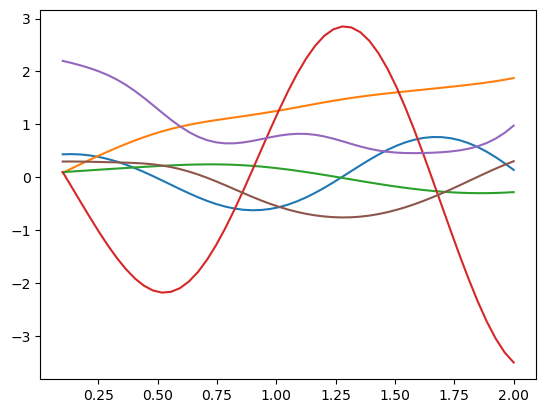
This plot shows that the state trajectory changes with respect to time, but
without some more information it is hard to interpret. The following function
uses subplots() to make a figure with
panels for the different state variables. I use
vlatex() to include the
symbolic symbol names in the legends. The other matplotlib functions and
methods I use are:
set_size_inches(),
plot(),
legend(),
set_ylabel(),
set_xlabel(), and
tight_layout().
I also make use of array slicing notation to select which rows and columns I want from each array. See the NumPy documentation Indexing on ndarrays for information on how this works.
def plot_results(ts, xs):
"""Returns the array of axes of a 4 panel plot of the state trajectory
versus time.
Parameters
==========
ts : array_like, shape(m,)
Values of time.
xs : array_like, shape(m, 6)
Values of the state trajectories corresponding to ``ts`` in order
[q1, q2, q3, u1, u2, u3].
Returns
=======
axes : ndarray, shape(4,)
Matplotlib axes for each panel.
"""
fig, axes = plt.subplots(4, 1, sharex=True)
fig.set_size_inches((10.0, 6.0))
axes[0].plot(ts, np.rad2deg(xs[:, :2]))
axes[1].plot(ts, xs[:, 2])
axes[2].plot(ts, np.rad2deg(xs[:, 3:5]))
axes[3].plot(ts, xs[:, 5])
axes[0].legend([me.vlatex(q[0], mode='inline'),
me.vlatex(q[1], mode='inline')])
axes[1].legend([me.vlatex(q[2], mode='inline')])
axes[2].legend([me.vlatex(u[0], mode='inline'),
me.vlatex(u[1], mode='inline')])
axes[3].legend([me.vlatex(u[2], mode='inline')])
axes[0].set_ylabel('Angle [deg]')
axes[1].set_ylabel('Distance [m]')
axes[2].set_ylabel('Angular Rate [deg/s]')
axes[3].set_ylabel('Speed [m/s]')
axes[3].set_xlabel('Time [s]')
fig.tight_layout()
return axes
Our function now gives an interpretable view of the results:
plot_results(ts, xs);
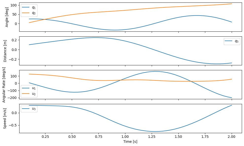
We now see that \(q_1\) oscillates between \(\pm 40 \textrm{deg}\) with a single period. \(q_2\) grows to around \(100 \textrm{deg}\), and \(q_3\) has half an oscillation period ranging between -0.2 and 0.2 meters. For the initial conditions and constants we choose, this seems physically feasible.
Integration with SciPy
Our euler_integrate() function seems to do the trick, but all numerical
integrators suffer from two types of errors: truncation error and floating
point arithmetic error. Truncation error is the dominant error and is due to
having to integrate over finite integration steps with approximations to the
area under the integral’s curve. Paying careful attention to truncation error
is needed to keep the error in the resulting trajectories within some
acceptable tolerance, usually close in magnitude to the floating point
arithmetic error. Euler’s Method has poor truncation error unless very small
time steps are chosen. But more time steps results in longer computation time.
There are a large number of other numerical integration methods that provide
better results with fewer time steps, but at the cost of more complexity in the
integration algorithm.
SciPy is built on top of NumPy and provides a large assortment of battle
tested numerical methods for NumPy arrays, including numerical methods for
integration. We are solving the initial value problem of ordinary differential
equations and SciPy includes the function
solve_ivp() for this purpose.
solve_ivp() provides access to a several different integration methods that
are suitable for different problems. The default method used is a Runge-Kutta
method that works well for non-stiff problems.
We will only be using solve_ivp() from SciPy so we can import it directly
with:
from scipy.integrate import solve_ivp
We can use solve_ivp() in much the same way as our euler_integrate()
function (in fact I designed euler_integrate() to mimic solve_ivp()).
The difference is that solve_ivp() takes a function that evaluates the
right hand side of the ordinary differential equations that is of the form
f(t, x) (no p!). Our parameter vector p must be passed to the
args= optional keyword argument in solve_ivp() to get things to work.
If we only have one extra argument, as we do f(t, x, p), then we must make
a 1-tuple (p_vals,). Other than that, the inputs are the same as
euler_integrate(). solve_ivp() returns a solution object that contains
quite a bit of information (other than the trajectories). See the documentation
for solve_ivp() for all the details and more
examples.
Here is how we use the integrator with our previously defined system:
result = solve_ivp(eval_rhs, (t0, tf), x0, args=(p_vals,))
The time values are in the result.t attribute:
result.t
array([0.1 , 0.13120248, 0.29762659, 0.54422251, 0.80410512,
1.06256808, 1.31993114, 1.57487353, 1.83715709, 2. ])
and the state trajectory is in the result.y attribute:
result.y
array([[ 0.43633231, 0.4358189 , 0.31525018, -0.11015295, -0.46375645,
-0.34485627, 0.12132567, 0.43601266, 0.27143017, -0.01911091],
[ 0.08726646, 0.15537688, 0.49605864, 0.88149593, 1.13596246,
1.39359322, 1.67416762, 1.92225131, 2.13926064, 2.29230085],
[ 0.1 , 0.10935888, 0.15799993, 0.21797738, 0.21721945,
0.11520445, -0.03955252, -0.17887644, -0.25034975, -0.24594355],
[ 0.1 , -0.13284291, -1.26834506, -1.88255608, -0.55453818,
1.39013663, 1.86357587, 0.37219434, -1.5003001 , -1.93004498],
[ 2.2 , 2.16517843, 1.90078084, 1.19931529, 0.90164316,
1.09025742, 1.04941978, 0.88566504, 0.83634928, 1.07386933],
[ 0.3 , 0.299615 , 0.28218305, 0.16978927, -0.2076191 ,
-0.54349971, -0.61398805, -0.44313122, -0.08440758, 0.13024152]])
Note the shape of the trajectory array:
np.shape(result.y)
It is the transpose of our xs computed above. Knowing that we can use our
plot_results() function to view the results. I use
transpose() to transpose the array before passing it
into the plot function.
plot_results(result.t, np.transpose(result.y));
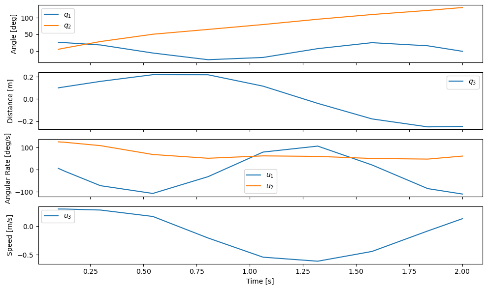
The default result is very coarse in time (only 10 time steps!). This is because the underlying integration algorithm adaptively selects the necessary time steps to stay within the desired maximum truncation error. The Runge-Kutta method gives good accuracy with fewer integration steps in this case.
If you want to specify which time values you’d like the result presented at you
can do so by interpolating the results by providing the time values with the
keyword argument t_eval=.
result = solve_ivp(eval_rhs, (t0, tf), x0, args=(p_vals,), t_eval=ts)
plot_results(result.t, np.transpose(result.y));
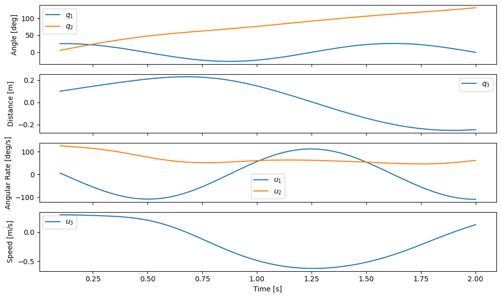
Lastly, let’s compare the results from euler_integrate() with
solve_ivp(), the later of which uses a Runge-Kutta method that has lower
truncation error. We’ll plot only \(q_1\) for this comparison. Note that
the two results for \(q_1\) are not the same, showing up to 20 degrees of
error:
np.rad2deg(xs[:, 0] - np.transpose(result.y)[:, 0])
array([ 0. , 0.30870206, 0.61345799, 0.89659378, 1.13980409,
1.32347734, 1.42776194, 1.43501062, 1.33083232, 1.10515873,
0.75190507, 0.2678 , -0.34841153, -1.07897973, -1.9073999 ,
-2.81131639, -3.76035282, -4.71997026, -5.65476872, -6.52908614,
-7.30042903, -7.9399897 , -8.41991318, -8.71098105, -8.78301005,
-8.60522949, -8.1508501 , -7.4106676 , -6.37961884, -5.06396319,
-3.48079062, -1.65574424, 0.3803268 , 2.58126391, 4.88311817,
7.2270935 , 9.54739236, 11.7758927 , 13.84593049, 15.69455704,
17.25818069, 18.48906606, 19.34750848, 19.7955033 , 19.7963994 ,
19.31507318, 18.31959642, 16.80072491, 14.76173147, 12.21963721,
9.21004694])
fig, ax = plt.subplots()
fig.set_size_inches((10.0, 6.0))
ax.plot(ts, np.rad2deg(xs[:, 0]), 'k',
result.t, np.rad2deg(np.transpose(result.y)[:, 0]), 'b');
ax.legend(['euler_integrate', 'solve_ivp'])
ax.set_xlabel('Time [s]')
ax.set_ylabel('Angle [deg]');
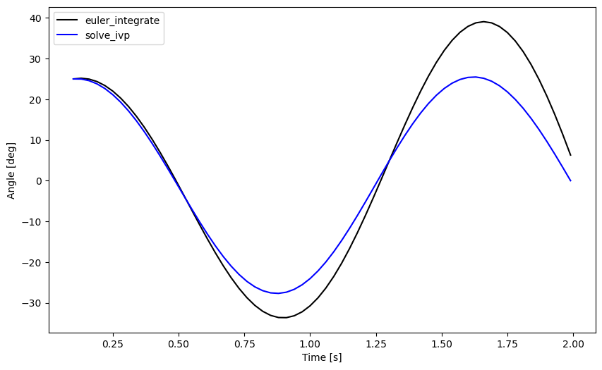
You can clearly see that the Euler Method deviates from the more accurate Runge-Kutta method. You’ll need to learn more about truncation error and the various integration methods to ensure you are getting the results you desire. For now, be aware that truncation error and floating point arithmetic error can give you inaccurate results.
Now set xs equal to the solve_ivp() result for use in the next section:
xs = np.transpose(result.y)
Animation with Matplotlib
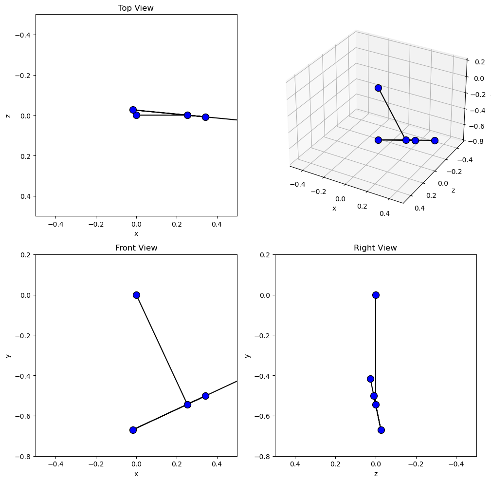
Matplotlib also provides tools to make animations by iterating over data and updating the plot. I’ll create a very simple set of plots that give 4 views of interesting points in our system.
Matplotlib’s plot axes default to displaying the abscissa (\(x\)) horizontal and positive towards the right and the ordinate (\(y\)) vertical and positive upwards. The coordinate system in Fig. 47 has \(\hat{n}_x\) positive downwards and \(\hat{n}_y\) positive to the right. We can create a viewing reference frame \(M\) that matches matplotlib’s axes like so:
M = me.ReferenceFrame('M')
M.orient_axis(N, sm.pi/2, N.z)
Now \(\hat{m}_x\) is positive to the right, \(\hat{m}_y\) is positive upwards, and \(\hat{m}_z\) points out of the screen.
I’ll also introduce a couple of points on each end of the rod \(B\), just for visualization purposes:
Bl = me.Point('B_l')
Br = me.Point('B_r')
Bl.set_pos(Bo, -l/2*B.y)
Br.set_pos(Bo, l/2*B.y)
Now, we can project the four points \(B_o,Q,B_l,B_r\) onto the unit vectors
of \(M\) using lambdify() to get the Cartesian coordinates of each
point relative to point \(O\). I use
row_join() to stack the
matrices together to build a single matrix with all points’ coordinates.
coordinates = O.pos_from(O).to_matrix(M)
for point in [Bo, Q, Bl, Br]:
coordinates = coordinates.row_join(point.pos_from(O).to_matrix(M))
eval_point_coords = sm.lambdify((q, p), coordinates)
eval_point_coords(q_vals, p_vals)
array([[ 0. , 0.25357096, 0.34385686, -0.01728675, 0.52442866],
[ 0. , -0.54378467, -0.50168367, -0.67008769, -0.41748165],
[ 0. , 0. , 0.00871557, -0.02614672, 0.02614672]])
The first row are the \(x\) coordinates of each point, the second row has the \(y\) coordinates, and the last the \(z\) coordinates.
Now create the desired 4 panel figure with three 2D views of the system and one
with a 3D view using the initial conditions and constant parameters shown. I
make use of add_subplot() to
control if the panel is 2D or 3D.
set_aspect() ensures that the abscissa
and ordinate dimensions display in a 1:1 ratio.
# initial configuration of the points
x, y, z = eval_point_coords(q_vals, p_vals)
# create a figure
fig = plt.figure()
fig.set_size_inches((10.0, 10.0))
# setup the subplots
ax_top = fig.add_subplot(2, 2, 1)
ax_3d = fig.add_subplot(2, 2, 2, projection='3d')
ax_front = fig.add_subplot(2, 2, 3)
ax_right = fig.add_subplot(2, 2, 4)
# common line and marker properties for each panel
line_prop = {
'color': 'black',
'marker': 'o',
'markerfacecolor': 'blue',
'markersize': 10,
}
# top view
lines_top, = ax_top.plot(x, z, **line_prop)
ax_top.set_xlim((-0.5, 0.5))
ax_top.set_ylim((0.5, -0.5))
ax_top.set_title('Top View')
ax_top.set_xlabel('x')
ax_top.set_ylabel('z')
ax_top.set_aspect('equal')
# 3d view
lines_3d, = ax_3d.plot(x, z, y, **line_prop)
ax_3d.set_xlim((-0.5, 0.5))
ax_3d.set_ylim((0.5, -0.5))
ax_3d.set_zlim((-0.8, 0.2))
ax_3d.set_xlabel('x')
ax_3d.set_ylabel('z')
ax_3d.set_zlabel('y')
# front view
lines_front, = ax_front.plot(x, y, **line_prop)
ax_front.set_xlim((-0.5, 0.5))
ax_front.set_ylim((-0.8, 0.2))
ax_front.set_title('Front View')
ax_front.set_xlabel('x')
ax_front.set_ylabel('y')
ax_front.set_aspect('equal')
# right view
lines_right, = ax_right.plot(z, y, **line_prop)
ax_right.set_xlim((0.5, -0.5))
ax_right.set_ylim((-0.8, 0.2))
ax_right.set_title('Right View')
ax_right.set_xlabel('z')
ax_right.set_ylabel('y')
ax_right.set_aspect('equal')
fig.tight_layout()
Now we will use FuncAnimation to
generate an animation. See the animation examples for more information on
creating animations with matplotib.
First import FuncAnimation():
from matplotlib.animation import FuncAnimation
Now create a function that takes an frame index i, calculates the
configuration of the points for the ith state in xs, and updates
the data for the lines we have already plotted with
set_data() and
set_data_3d().
def animate(i):
x, y, z = eval_point_coords(xs[i, :3], p_vals)
lines_top.set_data(x, z)
lines_3d.set_data_3d(x, z, y)
lines_front.set_data(x, y)
lines_right.set_data(z, y)
Now provide the figure, the animation update function, and the number of frames
to FuncAnimation:
ani = FuncAnimation(fig, animate, len(ts))
FuncAnimation can create an interactive animation, movie files, and other
types of outputs. Here I take advantage of IPython’s HTML display function and
the to_jshtml() method to
create a web browser friendly visualization of the animation.
from IPython.display import HTML
HTML(ani.to_jshtml(fps=30))
If we’ve setup our animation correctly and our equations of motion are correct, we should see physically believable motion of our system. In this case, it looks like we’ve successfully simulated and visualized our first multibody system!