Equations of Motion with Holonomic Constraints

Note

You can download this example as a Python script: holonomic-eom.py or Jupyter Notebook: holonomic-eom.ipynb.

from IPython.display import HTML
from matplotlib.animation import FuncAnimation
from scipy.integrate import solve_ivp
import matplotlib.pyplot as plt
import numpy as np
import sympy as sm
import sympy.physics.mechanics as me

me.init_vprinting(use_latex='mathjax')

class ReferenceFrame(me.ReferenceFrame):

    def __init__(self, *args, **kwargs):

        kwargs.pop('latexs', None)

        lab = args[0].lower()
        tex = r'\hat{{{}}}_{}'

        super(ReferenceFrame, self).__init__(*args,
                                             latexs=(tex.format(lab, 'x'),
                                                     tex.format(lab, 'y'),
                                                     tex.format(lab, 'z')),
                                             **kwargs)
me.ReferenceFrame = ReferenceFrame

Learning Objectives

After completing this chapter readers will be able to:

• formulate the differential algebraic equations of motion for a multibody system that includes additional holonomic constraints

• simulate a system with additional constraints using a differential algebraic equation integrator

• compare simulation results that do and do not manage constraint drift

Introduction

When there are holonomic constraints present the equations of motion are comprised of the kinematical differential equations \(\bar{f}_k=0\), dynamical differential equations \(\bar{f}_d=0\), and the holonomic constraint equations \(\bar{f}_h=0\). This set of equations are called differential algebraic equations and the algebraic equations cannot be solved for explicitly, as we did with the nonholonomic algebraic constraint equations.

In a system such as this, there are \(N=n+M\) total coordinates, with \(n\) generalized coordinates \(\bar{q}\) and \(M\) additional dependent coordinates \(\bar{q}_r\). The holonomic constraints take this form:

(207)\[\bar{f}_h(\bar{q}, \bar{q}_r, t) = 0 \in \mathbb{R}^M\]

\(n\) generalized speeds \(\bar{u}\) and \(M\) dependent speeds \(\bar{u}_r\) can be introduced using \(N\) kinematical differential equations.

(208)\[\begin{split}\bar{f}_k(\dot{\bar{q}}, \dot{\bar{q}}_r, \bar{u}, \bar{u}_r, \bar{q}, \bar{q}_r, t) = 0 \in \mathbb{R}^N \\\end{split}\]

We can formulate the equations of motion by transforming the holonomic constraints into a function of generalized speeds. These equations are then treated just like nonholonomic constraints described in the previous Chp. Equations of Motion with Nonholonomic Constraints.

(209)\[\dot{\bar{f}}_h(\bar{u}, \bar{u}_r, \bar{q}, \bar{q}_r, t) = \mathbf{M}_{hd}\bar{u}_r + \bar{g}_{hd} = 0 \in \mathbb{R}^M\]

We can solve for \(M\) dependent generalized speeds:

(210)\[\bar{u}_r = -\mathbf{M}_{hd}^{-1} \bar{g}_{hd} \in \mathbb{R}^M\]

and then rewrite the kinematical and dynamical differential equations in terms of the generalized speeds, their time derivatives, the generalized coordinates, and the dependent coordinates.

(211)\[\begin{split}\bar{f}_k(\dot{\bar{q}}, \dot{\bar{q}}_r, \bar{u}, \bar{q}, \bar{q}_r, t) = 0 \in \mathbb{R}^N \\ \bar{f}_d(\dot{\bar{u}}, \bar{u}, \bar{q}, \bar{q}_r, t) = 0 \in \mathbb{R}^n \\\end{split}\]

This final set of equations has \(N+n\) state variables and can be integrated as a set of ordinary differential equations or the \(N+n+M\) equations can be integrated as a set of differential algebraic equations. We will demonstrate the differences in the results for the two approaches.

Four-bar Linkage Equations of Motion

To demonstrate the formulation of the equations of motion of a system with an explicit holonomic constraints, let’s revisit the four-bar linkage from Sec. Four-Bar Linkage. We will now make \(P_2\) and \(P_3\) particles, each with mass \(m\) and include the effects of gravity in the \(-\hat{n}_y\) direction.

Fig. 49 a) Shows four links in a plane \(A\), \(B\), \(C\), and \(N\) with respective lengths \(l_a,l_b,l_c,l_n\) connected in a closed loop at points \(P_1,P_2,P_3,P_4\). b) Shows the same linkage that has been separated at point \(P_4\) to make it an open chain of links.

As before, we setup the system by disconnecting the kinematic loop at point \(P_4\) and then use this open loop to derive equations for the holonomic constraints that close the loop.

1. Declare all of the variables

We have three coordinates, only one of which is a generalized coordinate. I use q to hold the single generalized coordinate, qr for the two dependent coordinates, and qN to hold all the coordinates; similarly for the generalized speeds.

q1, q2, q3 = me.dynamicsymbols('q1, q2, q3')
u1, u2, u3 = me.dynamicsymbols('u1, u2, u3')
la, lb, lc, ln = sm.symbols('l_a, l_b, l_c, l_n')
m, g = sm.symbols('m, g')
t = me.dynamicsymbols._t

p = sm.Matrix([la, lb, lc, ln, m, g])

q = sm.Matrix([q1])
qr = sm.Matrix([q2, q3])
qN = q.col_join(qr)

u = sm.Matrix([u1])
ur = sm.Matrix([u2, u3])
uN = u.col_join(ur)

qdN = qN.diff(t)
ud = u.diff(t)

p, q, qr, qN, u, ur, uN, qdN, ud

\[\begin{split}\displaystyle \left( \left[\begin{matrix}l_{a}\\l_{b}\\l_{c}\\l_{n}\\m\\g\end{matrix}\right], \ \left[\begin{matrix}q_{1}\end{matrix}\right], \ \left[\begin{matrix}q_{2}\\q_{3}\end{matrix}\right], \ \left[\begin{matrix}q_{1}\\q_{2}\\q_{3}\end{matrix}\right], \ \left[\begin{matrix}u_{1}\end{matrix}\right], \ \left[\begin{matrix}u_{2}\\u_{3}\end{matrix}\right], \ \left[\begin{matrix}u_{1}\\u_{2}\\u_{3}\end{matrix}\right], \ \left[\begin{matrix}\dot{q}_{1}\\\dot{q}_{2}\\\dot{q}_{3}\end{matrix}\right], \ \left[\begin{matrix}\dot{u}_{1}\end{matrix}\right]\right)\end{split}\]

ur_zero = {ui: 0 for ui in ur}
uN_zero = {ui: 0 for ui in uN}
qdN_zero = {qdi: 0 for qdi in qdN}
ud_zero = {udi: 0 for udi in ud}

2. Setup the open loop kinematics and holonomic constraints

Start by defining the orientation of the reference frames and positions of the points in terms of the \(N=3\) coordinates, leaving \(P_4\) unconstrained.

N = me.ReferenceFrame('N')
A = me.ReferenceFrame('A')
B = me.ReferenceFrame('B')
C = me.ReferenceFrame('C')

A.orient_axis(N, q1, N.z)
B.orient_axis(A, q2, A.z)
C.orient_axis(B, q3, B.z)

P1 = me.Point('P1')
P2 = me.Point('P2')
P3 = me.Point('P3')
P4 = me.Point('P4')

P2.set_pos(P1, la*A.x)
P3.set_pos(P2, lb*B.x)
P4.set_pos(P3, lc*C.x)

3. Create the holonomic constraints

Now \(M=2\) holonomic constraints can be found by closing the loop.

loop = P4.pos_from(P1) - ln*N.x

fh = sm.Matrix([loop.dot(N.x), loop.dot(N.y)])
fh = sm.trigsimp(fh)
fh

\[\begin{split}\displaystyle \left[\begin{matrix}l_{a} \cos{\left(q_{1} \right)} + l_{b} \cos{\left(q_{1} + q_{2} \right)} + l_{c} \cos{\left(q_{1} + q_{2} + q_{3} \right)} - l_{n}\\l_{a} \sin{\left(q_{1} \right)} + l_{b} \sin{\left(q_{1} + q_{2} \right)} + l_{c} \sin{\left(q_{1} + q_{2} + q_{3} \right)}\end{matrix}\right]\end{split}\]

Warning

Be careful about using trigsimp() on larger problems, as it can really slow down the calculations. It is not necessary to use, but I do so here so that the resulting equations are human readable in this context.

Note that these constraints are only a function of the \(N\) coordinates, not their time derivatives.

me.find_dynamicsymbols(fh)

\[\displaystyle \left\{q_{1}, q_{2}, q_{3}\right\}\]

4. Specify the kinematical differential equations

Use simple definitions for the generalized speed \(u_1\) and the dependent speeds \(u_2\) and \(u_3\). We create \(N=3\) generalized speeds even though the degrees of freedom are \(n=1\).

fk = sm.Matrix([
    q1.diff(t) - u1,
    q2.diff(t) - u2,
    q3.diff(t) - u3,
])
Mk = fk.jacobian(qdN)
gk = fk.xreplace(qdN_zero)
qdN_sol = -Mk.LUsolve(gk)
qd_repl = dict(zip(qdN, qdN_sol))
qd_repl

\[\displaystyle \left\{ \dot{q}_{1} : u_{1}, \ \dot{q}_{2} : u_{2}, \ \dot{q}_{3} : u_{3}\right\}\]

5. Solve for the dependent speeds

Differentiate the holonomic constraints with respect to time to arrive at a motion constraint. This is equivalent to setting \(^{N}\bar{v}^{P_4}=0\).

fhd = fh.diff(t).xreplace(qd_repl)
fhd = sm.trigsimp(fhd)
fhd

\[\begin{split}\displaystyle \left[\begin{matrix}- l_{a} u_{1} \sin{\left(q_{1} \right)} - l_{b} \left(u_{1} + u_{2}\right) \sin{\left(q_{1} + q_{2} \right)} - l_{c} \left(u_{1} + u_{2} + u_{3}\right) \sin{\left(q_{1} + q_{2} + q_{3} \right)}\\l_{a} u_{1} \cos{\left(q_{1} \right)} + l_{b} \left(u_{1} + u_{2}\right) \cos{\left(q_{1} + q_{2} \right)} + l_{c} \left(u_{1} + u_{2} + u_{3}\right) \cos{\left(q_{1} + q_{2} + q_{3} \right)}\end{matrix}\right]\end{split}\]

These holonomic motion constraints are functions of the coordinates and speeds.

me.find_dynamicsymbols(fhd)

\[\displaystyle \left\{q_{1}, q_{2}, q_{3}, u_{1}, u_{2}, u_{3}\right\}\]

Choose \(u_2\) and \(u_3\) as the dependent speeds and solve the linear equations for these dependent speeds.

Mhd = fhd.jacobian(ur)
ghd = fhd.xreplace(ur_zero)
ur_sol = sm.trigsimp(-Mhd.LUsolve(ghd))
ur_repl = dict(zip(ur, ur_sol))
ur_repl[u2]

\[\displaystyle \frac{- l_{a} u_{1} \sin{\left(q_{1} \right)} - \frac{l_{a} \left(l_{b} \sin{\left(q_{2} \right)} + l_{c} \sin{\left(q_{2} + q_{3} \right)}\right) u_{1} \sin{\left(q_{1} + q_{2} + q_{3} \right)}}{l_{b} \sin{\left(q_{3} \right)}} - l_{b} u_{1} \sin{\left(q_{1} + q_{2} \right)} - l_{c} u_{1} \sin{\left(q_{1} + q_{2} + q_{3} \right)}}{l_{b} \sin{\left(q_{1} + q_{2} \right)} + l_{c} \sin{\left(q_{1} + q_{2} + q_{3} \right)}}\]

ur_repl[u3]

\[\displaystyle \frac{l_{a} \left(l_{b} \sin{\left(q_{2} \right)} + l_{c} \sin{\left(q_{2} + q_{3} \right)}\right) u_{1}}{l_{b} l_{c} \sin{\left(q_{3} \right)}}\]

6. Write velocities in terms of the generalized speeds

We have three simple rotations and we can write the three angular velocities only in terms of \(u_1\) by using the expressions for the independent speeds from the previous step.

A.set_ang_vel(N, u1*N.z)
B.set_ang_vel(A, ur_repl[u2]*A.z)
C.set_ang_vel(B, ur_repl[u3]*B.z)

Now, by using the two point velocity theorem the velocities of each point will also only be in terms of \(u_1\).

P1.set_vel(N, 0)
P2.v2pt_theory(P1, N, A)
P3.v2pt_theory(P2, N, B)
P4.v2pt_theory(P3, N, C)

(me.find_dynamicsymbols(P2.vel(N), reference_frame=N) |
 me.find_dynamicsymbols(P3.vel(N), reference_frame=N) |
 me.find_dynamicsymbols(P4.vel(N), reference_frame=N))

\[\displaystyle \left\{q_{1}, q_{2}, q_{3}, u_{1}\right\}\]

We’ll also need the kinematical differential equations only in terms of the one generalized speed \(u_1\), so replace the dependent speeds in \(\bar{g}_k\).

gk = gk.xreplace(ur_repl)

7. Form the generalized active forces

We have a holonomic system so the number of degrees of freedom is \(n=1\). There are two particles that move and gravity acts on each of them, as a contributing force. The resultant contributing forces on each of the particles are:

R_P2 = -m*g*N.y
R_P3 = -m*g*N.y

The partial velocities of each particle are easily found for the single generalized speed and \(\bar{F}_r\) is:

Fr = sm.Matrix([
    P2.vel(N).diff(u1, N).dot(R_P2) + P3.vel(N).diff(u1, N).dot(R_P3)
])
Fr

\[\displaystyle \left[\begin{matrix}- 2 g l_{a} m \cos{\left(q_{1} \right)} - g l_{b} m \left(1 + \frac{- l_{a} \sin{\left(q_{1} \right)} - \frac{l_{a} \left(l_{b} \sin{\left(q_{2} \right)} + l_{c} \sin{\left(q_{2} + q_{3} \right)}\right) \sin{\left(q_{1} + q_{2} + q_{3} \right)}}{l_{b} \sin{\left(q_{3} \right)}} - l_{b} \sin{\left(q_{1} + q_{2} \right)} - l_{c} \sin{\left(q_{1} + q_{2} + q_{3} \right)}}{l_{b} \sin{\left(q_{1} + q_{2} \right)} + l_{c} \sin{\left(q_{1} + q_{2} + q_{3} \right)}}\right) \left(- \sin{\left(q_{1} \right)} \sin{\left(q_{2} \right)} + \cos{\left(q_{1} \right)} \cos{\left(q_{2} \right)}\right)\end{matrix}\right]\]

Check to make sure our generalized active forces do not contain dependent speeds.

me.find_dynamicsymbols(Fr)

\[\displaystyle \left\{q_{1}, q_{2}, q_{3}\right\}\]

8. Form the generalized inertia forces

To calculate the generalized inertia forces we need the acceleration of each particle. These should be only functions of \(\dot{u}_1,u_1\), and the three coordinates. For \(P_2\), that is already true:

me.find_dynamicsymbols(P2.acc(N), reference_frame=N)

\[\displaystyle \left\{q_{1}, u_{1}, \dot{u}_{1}\right\}\]

but for \(P_3\) we need to make some substitutions:

me.find_dynamicsymbols(P3.acc(N), reference_frame=N)

\[\displaystyle \left\{q_{1}, q_{2}, q_{3}, u_{1}, \dot{q}_{1}, \dot{q}_{2}, \dot{q}_{3}, \dot{u}_{1}\right\}\]

Knowing that, the inertia resultants can be written as:

Rs_P2 = -m*P2.acc(N)
Rs_P3 = -m*P3.acc(N).xreplace(qd_repl).xreplace(ur_repl)

and the generalized inertia forces can be formed and we can make sure they are not functions of the dependent speeds.

Frs = sm.Matrix([
    P2.vel(N).diff(u1, N).dot(Rs_P2) + P3.vel(N).diff(u1, N).dot(Rs_P3)
])
me.find_dynamicsymbols(Frs)

\[\displaystyle \left\{q_{1}, q_{2}, q_{3}, u_{1}, \dot{u}_{1}\right\}\]

9. Equations of motion

Finally, the matrix form of dynamical differential equations is found as we have done before.

Md = Frs.jacobian(ud)
gd = Frs.xreplace(ud_zero) + Fr

And we can check to make sure the dependent speeds have been eliminated.

me.find_dynamicsymbols(Mk), me.find_dynamicsymbols(gk)

\[\displaystyle \left( \left\{\right\}, \ \left\{q_{1}, q_{2}, q_{3}, u_{1}\right\}\right)\]

me.find_dynamicsymbols(Md), me.find_dynamicsymbols(gd)

\[\displaystyle \left( \left\{q_{1}, q_{2}, q_{3}\right\}, \ \left\{q_{1}, q_{2}, q_{3}, u_{1}\right\}\right)\]

Simulate without constraint enforcement

The equations of motion are functions of all three coordinates, yet two of them are dependent on the other. For the evaluation of the right hand side of the equations to be valid, the coordinates must satisfy the holonomic constraints. As presented, Eqs. (211) only contain the constraints that the velocity and acceleration of point \(P_4\) must be zero, but the position constraint is not explicitly present. Neglecting the position constraint will cause numerical issues during integration, as we will see.

Create an eval_rhs(t, x, p) as we have done before, noting that \(\bar{f}_d \in \mathbb{R}^1\).

eval_k = sm.lambdify((qN, u, p), (Mk, gk))
eval_d = sm.lambdify((qN, u, p), (Md, gd))


def eval_rhs(t, x, p):
    """Return the derivative of the state at time t.

    Parameters
    ==========
    t : float
    x : array_like, shape(4,)
       x = [q1, q2, q3, u1]
    p : array_like, shape(6,)
       p = [la, lb, lc, ln, m, g]

    Returns
    =======
    xd : ndarray, shape(4,)
       xd = [q1d, q2d, q3d, u1d]

    """

    qN = x[:3]  # shape(3,)
    u = x[3:]   # shape(1,)

    Mk, gk = eval_k(qN, u, p)
    qNd = -np.linalg.solve(Mk, np.squeeze(gk))

    # Md, gd, and ud are each shape(1,1)
    Md, gd = eval_d(qN, u, p)
    ud = -np.linalg.solve(Md, gd)[0]

    return np.hstack((qNd, ud))

Here I select some feasible bar lengths. See the section on the Grashof condition to learn more about selecting lengths in four-bar linkages.

p_vals = np.array([
    0.8,  # la [m]
    2.0,  # lb [m]
    1.0,  # lc [m]
    2.0,  # ln [m]
    1.0,  # m [kg]
    9.81,  # g [m/s^2]
])

Now we need to generate coordinates that are consistent with the constraints. \(\bar{f}_h\) is nonlinear in all of the coordinates. We can solve these equations for the dependent coordinates using numerical root finding methods. SciPy’s fsolve() function is capable of finding the roots for sets of nonlinear equations, given a good guess.

We’ll import fsolve directly like so:

from scipy.optimize import fsolve

fsolve() requires a function that evaluates expressions that equal to zero and a guess for the roots of that function, at a minimum. Nonlinear functions will most certianly have multiple solutions for its roots and fsolve() will converge to one of the solutions. The better the provided the guess the more likely it will converge on the desired solution. Our function should evaluate the holonomic constraints given the dependent coordinates. We can use lambdify() to create this function. I make the first argument \(\bar{q}_r\) because these are the values we want to solve for using fsolve().

eval_fh = sm.lambdify((qr, q1, p), fh)

Now select a desired value for the generalized coordinate \(q_1\) and guesses for \(q_2\) and \(q_3\).

q1_val = np.deg2rad(10.0)
qr_guess = np.deg2rad([10.0, -150.0])

eval_fh() returns a 2x1 array so a lambda function is used to squeeze the output. \(q_2\) and \(q_3\) that satisfy the constraints are then found with:

q2_val, q3_val = fsolve(
    lambda qr, q1, p: np.squeeze(eval_fh(qr, q1, p)),  # squeeze to a 1d array
    qr_guess,  # initial guess for q2 and q3
    args=(q1_val, p_vals)) # known values in fh

Now we have values of the coordinates that satisfy the constraints.

qN_vals = np.array([q1_val, q2_val, q3_val])
np.rad2deg(qN_vals)

array([  10.        ,    6.57526576, -151.3836336 ])

We can check that they return zero (or better stated as within fsolve()’s tolerance):

eval_fh(qN_vals[1:], qN_vals[0], p_vals)

array([[-2.44249065e-14],
       [ 5.88751270e-13]])

Exercise

There are most often multiple solutions for the dependent coordinates for a given value of the dependent coordinates. What are the other possible solutions for these parameter values?

Now that we have consistent coordinates, the initial state vector can be created. We will start at an initial state of rest with \(u_1(t_0)=0\).

u1_val = 0.0
x0 = np.hstack((qN_vals, u1_val))
x0

array([ 0.17453293,  0.11476004, -2.64214284,  0.        ])

We will integrate over 30 seconds to show how the constraints hold up over a longer period of time.

t0, tf, fps = 0.0, 30.0, 20

With consistent coordinates the initial conditions can be set and eval_rhs() tested.

eval_rhs(t0, x0, p_vals)

array([ 0.       , -0.       , -0.       , -9.4688079])

At every time step in the simulation the holonomic constraints should be satisfied. To check this we will need to evaluate the constraints \(\bar{f}_h\) at each time step. The following function does this and returns the constraint residuals at each time step.

def eval_constraints(xs, p):
    """Returns the value of the left hand side of the holonomic constraints
    at each time instance.

    Parameters
    ==========
    xs : ndarray, shape(n, 4)
        States at each of n time steps.
    p : ndarray, shape(6,)
        Constant parameters.

    Returns
    =======
    con : ndarray, shape(n, 2)
        fh evaluated at each xi in xs.

    """
    con = []
    for xi in xs:  # xs is shape(n, 4)
       con.append(eval_fh(xi[1:3], xi[0], p).squeeze())
    return np.array(con)

The dependent initial conditions need to be solved before each simulation and the constraints evaluated, so it will be helpful to package this process into a reusable function. The following function takes the simulation parameters and returns the simulation results. I have set the integration tolerances explicitly as rtol=1e-3 and atol=1e-6. These happen to be the default tolerances for solve_ivp() and we will use three different approaches and we want to make sure the tolerances are set the same for each integration so we can fairly compare the results.

def simulate(eval_rhs, t0, tf, fps, q1_0, u1_0, q2_0g, q3_0g, p):
    """Returns the simulation results.

    Parameters
    ==========
    eval_rhs : function
       Function that returns the derivatives of the states in the form:
       ``eval_rhs(t, x, p)``.
    t0 : float
       Initial time in seconds.
    tf : float
       Final time in seconds.
    fps : integer
       Number of "frames" per second to output.
    q1_0 : float
       Initial q1 angle in radians.
    u1_0 : float
       Initial u1 rate in radians/s.
    q2_0g : float
       Guess for the initial q2 angle in radians.
    q3_0g : float
       Guess for the initial q3 angle in radians.
    p : array_like, shape(6,)
       Constant parameters p = [la, lb, lc, ln, m, g].

    Returns
    =======
    ts : ndarray, shape(n,)
       Time values.
    xs : ndarray, shape(n, 4)
       State values at each time.
    con : ndarray, shape(n, 2)
       Constraint violations at each time in meters.

    """

    # generate the time steps
    ts = np.linspace(t0, tf, num=int(fps*(tf - t0)))

    # solve for the dependent coordinates
    q2_val, q3_val = fsolve(
        lambda qr, q1, p: np.squeeze(eval_fh(qr, q1, p)),
        [q2_0g, q3_0g],
        args=(q1_0, p))

    # establish the initial conditions
    x0 = np.array([q1_val, q2_val, q3_val, u1_0])

    # integrate the equations of motion
    sol = solve_ivp(eval_rhs, (ts[0], ts[-1]), x0, args=(p,), t_eval=ts,
                    rtol=1e-3, atol=1e-6)
    xs = np.transpose(sol.y)
    ts = sol.t

    # evaluate the constraints
    con = eval_constraints(xs, p)

    return ts, xs, con

Similarly, create a function that can be reused for plotting the state trajectories and the constraint residuals.

def plot_results(ts, xs, con):
    """Returns the array of axes of a 4 panel plot of the state trajectory
    versus time.

    Parameters
    ==========
    ts : array_like, shape(n,)
       Values of time.
    xs : array_like, shape(n, 4)
       Values of the state trajectories corresponding to ``ts`` in order
       [q1, q2, q3, u1].
    con : array_like, shape(n, 2)
       x and y constraint residuals of P4 at each time in ``ts``.

    Returns
    =======
    axes : ndarray, shape(3,)
       Matplotlib axes for each panel.

    """
    fig, axes = plt.subplots(3, 1, sharex=True)

    fig.set_size_inches((10.0, 6.0))

    axes[0].plot(ts, np.rad2deg(xs[:, :3]))  # q1(t), q2(t), q3(t)
    axes[1].plot(ts, np.rad2deg(xs[:, 3]))  # u1(t)
    axes[2].plot(ts, np.squeeze(con))  # fh(t)

    axes[0].legend(['$q_1$', '$q_2$', '$q_3$'])
    axes[1].legend(['$u_1$'])
    axes[2].legend([r'$\cdot\hat{n}_x$', r'$\cdot\hat{n}_y$'])

    axes[0].set_ylabel('Angle [deg]')
    axes[1].set_ylabel('Angular Rate [deg/s]')
    axes[2].set_ylabel('Distance [m]')
    axes[2].set_xlabel('Time [s]')

    fig.tight_layout()

    return axes

With the functions in place we can simulate the system and plot the results.

ts, xs, con = simulate(
    eval_rhs,
    t0=t0,
    tf=tf,
    fps=fps,
    q1_0=np.deg2rad(10.0),
    u1_0=0.0,
    q2_0g=np.deg2rad(10.0),
    q3_0g=np.deg2rad(-150.0),
    p=p_vals,
)
plot_results(ts, xs, con);

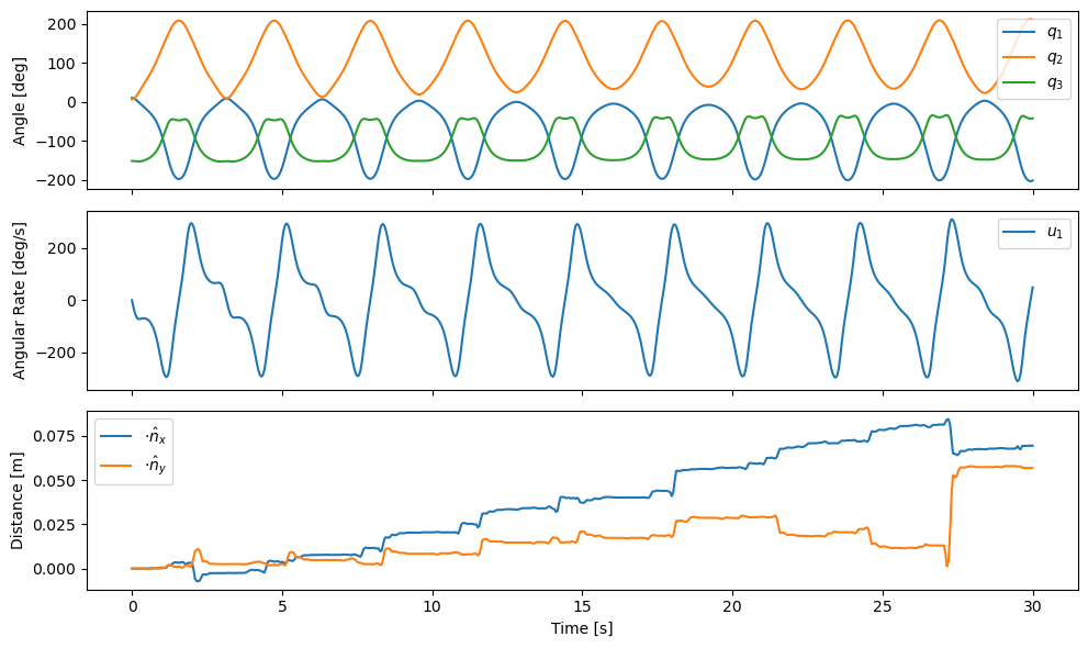
At first glance, the linkage seems to simulate fine with realistic angle values and angular rates. The motion is periodic but looking closely, for example at \(u_1(t)\), you can see that the angular rate changes in each successive period. The last graph shows the holonomic constraint residuals across time. This graph shows that the constraints are satisfied at the beginning of the simulation but that the residuals grow over time. This accumulation of error grows as large as 8 cm near the end of the simulation. The drifting constraint residuals are the cause of the variations of motion among the oscillation periods. Tighter integration tolerances can reduce the drifting constraint residuals, but that will come at an unnecessary computational cost and not fully solve the issue.

The effect of the constraints not staying satisfied throughout the simulation can also be seen if the system is animated.

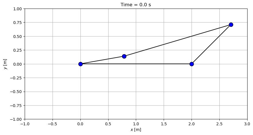
Animate the Motion

We’ll animate the four bar linkage multiple times so it is useful to create some functions to for the repeated use. Start by creating a function that evaluates the point locations, as we have done before.

coordinates = P2.pos_from(P1).to_matrix(N)
for point in [P3, P4, P1, P2]:
   coordinates = coordinates.row_join(point.pos_from(P1).to_matrix(N))
eval_point_coords = sm.lambdify((qN, p), coordinates)

Now create a function that plots the initial configuration of the linkage and returns any objects we may need in the animation code.

def setup_animation_plot(ts, xs, p):
    """Returns objects needed for the animation.

    Parameters
    ==========
    ts : array_like, shape(n,)
       Values of time.
    xs : array_like, shape(n, 4)
       Values of the state trajectories corresponding to ``ts`` in order
       [q1, q2, q3, u1].
    p : array_like, shape(6,)

    """

    x, y, z = eval_point_coords(xs[0, :3], p)

    fig, ax = plt.subplots()
    fig.set_size_inches((10.0, 10.0))
    ax.set_aspect('equal')
    ax.grid()

    lines, = ax.plot(x, y, color='black',
                     marker='o', markerfacecolor='blue', markersize=10)

    title_text = ax.set_title('Time = {:1.1f} s'.format(ts[0]))
    ax.set_xlim((-1.0, 3.0))
    ax.set_ylim((-1.0, 1.0))
    ax.set_xlabel('$x$ [m]')
    ax.set_ylabel('$y$ [m]')

    return fig, ax, title_text, lines

setup_animation_plot(ts, xs, p_vals);

Now we can create a function that initializes the plot, runs the animation and displays the results in Jupyter.

def animate_linkage(ts, xs, p):
    """Returns an animation object.

    Parameters
    ==========
    ts : array_like, shape(n,)
    xs : array_like, shape(n, 4)
       x = [q1, q2, q3, u1]
    p : array_like, shape(6,)
       p = [la, lb, lc, ln, m, g]

    """
    # setup the initial figure and axes
    fig, ax, title_text, lines = setup_animation_plot(ts, xs, p)

    # precalculate all of the point coordinates
    coords = []
    for xi in xs:
        coords.append(eval_point_coords(xi[:3], p))
    coords = np.array(coords)

    # define the animation update function
    def update(i):
        title_text.set_text('Time = {:1.1f} s'.format(ts[i]))
        lines.set_data(coords[i, 0, :], coords[i, 1, :])

    # close figure to prevent premature display
    plt.close()

    # create and return the animation
    return FuncAnimation(fig, update, len(ts))

Now, keep an eye on \(P_4\) during the animation of the simulation.

HTML(animate_linkage(ts, xs, p_vals).to_jshtml(fps=fps))

Once Loop Reflect