Orientation of Reference Frames

Note

You can download this example as a Python script: orientation.py or Jupyter Notebook: orientation.ipynb.

import sympy as sm
sm.init_printing(use_latex='mathjax')

Learning Objectives

After completing this chapter readers will be able to:

• Define a reference frame with associated unit vectors.

• Define a direction cosine matrix between two oriented reference frames.

• Derive direction cosine matrices for simple rotations.

• Derive direction cosine matrices for successive rotations.

• Manage orientation and direction cosine matrices with SymPy.

• Rotate reference frames using Euler Angles.

Reference Frames

In the study of multibody dynamics, we are interested in observing motion of connected and interacting objects in three dimensional space. This observation necessitates the concept of a frame of reference, or reference frame. A reference frame is an abstraction which we define as the set of all points in Euclidean space that are carried by and fixed to the observer of any given state of motion. Practically speaking, it is useful to imagine your eye as an observer of motion. Your eye can orient itself in 3D space to view the motion of objects from any direction and the motion of objects will appear differently in the set of points associated with the reference frame attached to your eye depending on your eye’s orientation.

It is important to note that a reference frame is not equivalent to a coordinate system. Any number of coordinate systems (e.g., Cartesian or spherical) can be used to describe the motion of points or objects in a reference frame. The coordinate system offers a system of measurement in a reference frame. We will characterize a reference frame by a right-handed set of mutually perpendicular unit vectors that can be used to describe its orientation relative to other reference frames and we will align a Cartesian coordinate system with the unit vectors to allow for easy measurement of points fixed or moving in the reference frame.

Unit Vectors

Vectors have a magnitude, direction, and sense (\(\pm\)) but notably not a position. Unit vectors have a magnitude of 1. Unit vectors can be fixed, orientation-wise, to a reference frame. For a reference frame named \(N\) we will define the three mutually perpendicular unit vectors as \(\hat{n}_x, \hat{n}_y, \hat{n}_z\) where these right-handed cross products hold:

(11)\[\begin{split}\hat{n}_x \times \hat{n}_y & = \hat{n}_z \\ \hat{n}_y \times \hat{n}_z & = \hat{n}_x \\ \hat{n}_z \times \hat{n}_x & = \hat{n}_y\end{split}\]

Note

Unit vectors will be designated using the “hat”, e.g. \(\hat{v}\).

These unit vectors are fixed in the reference frame \(N\). If a second reference frame \(A\) is defined, also with its set of right-handed mutually perpendicular unit vectors \(\hat{a}_x, \hat{a}_y, \hat{a}_z\) then we can establish the relative orientation of these two reference frames based on the angles among the two frames’ unit vectors.

Fig. 1 The image on the left and right represent the same set of right-handed mutually perpendicular unit vectors. Vectors, in general, do not have a position and can be drawn anywhere in the reference frame. Drawing them with their tails coincident is simply done for convenience.

Simple Orientations

Starting with two reference frames \(N\) and \(A\) in which their sets of unit vectors are initially aligned, the \(A\) frame can then be simply oriented about the common parallel \(z\) unit vectors of the two frames. We then say “reference frame \(A\) is oriented with respect to reference frame \(N\) about the shared \(z\) unit vectors through an angle \(\theta\). A visual representation of this orientation looking from the direction of the positive \(z\) unit vector is:

Fig. 2 View of the parallel \(xy\) planes of the simply oriented reference frames.

From the above figure these relationships between the \(\hat{a}\) and \(\hat{n}\) unit vectors can be deduced:

(12)\[\begin{split}\hat{a}_x & = \cos{\theta} \hat{n}_x + \sin{\theta} \hat{n}_y + 0 \hat{n}_z \\ \hat{a}_y & = -\sin{\theta} \hat{n}_x + \cos{\theta} \hat{n}_y + 0 \hat{n}_z \\ \hat{a}_z & = 0 \hat{n}_x + 0 \hat{n}_y + 1 \hat{n}_z\end{split}\]

These equations can also be written in a matrix form:

(13)\[\begin{split}\begin{bmatrix} \hat{a}_x \\ \hat{a}_y \\ \hat{a}_z \end{bmatrix} = \begin{bmatrix} \cos{\theta} & \sin{\theta} & 0 \\ -\sin{\theta} & \cos{\theta} & 0 \\ 0 & 0 & 1 \end{bmatrix} \begin{bmatrix} \hat{n}_x \\ \hat{n}_y \\ \hat{n}_z \end{bmatrix}\end{split}\]

This matrix uniquely describes the orientation between the two reference frames and so we give it its own variable:

(14)\[\begin{split}\begin{bmatrix} \hat{a}_x \\ \hat{a}_y \\ \hat{a}_z \end{bmatrix} = {}^A\mathbf{C}^N \begin{bmatrix} \hat{n}_x \\ \hat{n}_y \\ \hat{n}_z \end{bmatrix}\end{split}\]

This matrix \({}^A\mathbf{C}^N\) maps vectors expressed in the \(N\) frame to vectors expressed in the \(A\) frame. This matrix has an important property, which we will demonstrate with SymPy. Start by creating the matrix:

theta = sm.symbols('theta')

A_C_N = sm.Matrix([[sm.cos(theta), sm.sin(theta), 0],
                   [-sm.sin(theta), sm.cos(theta), 0],
                   [0, 0, 1]])
A_C_N

\[\begin{split}\displaystyle \left[\begin{matrix}\cos{\left(\theta \right)} & \sin{\left(\theta \right)} & 0\\- \sin{\left(\theta \right)} & \cos{\left(\theta \right)} & 0\\0 & 0 & 1\end{matrix}\right]\end{split}\]

If we’d like the inverse relationship between the two sets of unit vectors and \({}^A\mathbf{C}^N\) is invertible, then:

(15)\[\begin{split}\begin{bmatrix} \hat{n}_x \\ \hat{n}_y \\ \hat{n}_z \end{bmatrix} = \left({}^A\mathbf{C}^N\right)^{-1} \begin{bmatrix} \hat{a}_x \\ \hat{a}_y \\ \hat{a}_z \end{bmatrix}\end{split}\]

SymPy can find this matrix inverse:

sm.trigsimp(A_C_N.inv())

\[\begin{split}\displaystyle \left[\begin{matrix}\cos{\left(\theta \right)} & - \sin{\left(\theta \right)} & 0\\\sin{\left(\theta \right)} & \cos{\left(\theta \right)} & 0\\0 & 0 & 1\end{matrix}\right]\end{split}\]

SymPy can also find the transpose of this matrix;

A_C_N.transpose()

\[\begin{split}\displaystyle \left[\begin{matrix}\cos{\left(\theta \right)} & - \sin{\left(\theta \right)} & 0\\\sin{\left(\theta \right)} & \cos{\left(\theta \right)} & 0\\0 & 0 & 1\end{matrix}\right]\end{split}\]

Notably, the inverse and the transpose are the same here. This indicates that this matrix is a special orthogonal matrix. All matrices that describe the orientation between reference frames are orthogonal matrices. Following the notation convention, this holds:

(16)\[{}^N\mathbf{C}^A = \left({}^A\mathbf{C}^N\right)^{-1} = \left({}^A\mathbf{C}^N\right)^T\]

Exercise

Write \({}^A\mathbf{C}^N\) for simple rotations about both the shared \(\hat{n}_x\) and \(\hat{a}_x\) and shared \(\hat{n}_y\) and \(\hat{a}_y\) axes, rotating \(A\) with respect to \(N\) through angle \(\theta\).

Solution

For a \(x\) orientation:

(17)\[\begin{split}\begin{bmatrix} 1 & 0 & 0 \\ 0 & \cos{\theta} & \sin{\theta} \\ 0 & -\sin{\theta} & \cos{\theta} \end{bmatrix}\end{split}\]

For a \(y\) orientation:

(18)\[\begin{split}\begin{bmatrix} \cos{\theta} & 0 & -\sin{\theta} \\ 0 & 1 & 0 \\ \sin{\theta} & 0 & \cos{\theta} \end{bmatrix}\end{split}\]

Direction Cosine Matrices

If now \(A\) is oriented relative to \(N\) and the pairwise angles between each \(\hat{a}\) and \(\hat{n}\) mutually perpendicular unit vectors are measured, a matrix for an arbitrary orientation can be defined. For example, the figure below shows the three angles \(\alpha_{xx},\alpha_{xy},\alpha_{xz}\) relating \(\hat{a}_x\) to each \(\hat{n}\) unit vector.

Fig. 3 Three angles relating \(\hat{a}_x\) to the unit vectors of \(N\).

Similar to the simple example above, we can write these equations if the \(\alpha_y\) and \(\alpha_z\) angles relate the \(\hat{a}_y\) and \(\hat{a}_z\) unit vectors to those of \(N\):

(19)\[\begin{split}\hat{a}_x & = \cos\alpha_{xx} \hat{n}_x +\cos\alpha_{xy} \hat{n}_y + \cos\alpha_{xz} \hat{n}_z \\ \hat{a}_y & = \cos\alpha_{yx} \hat{n}_x +\cos\alpha_{yy} \hat{n}_y + \cos\alpha_{yz} \hat{n}_z \\ \hat{a}_z & = \cos\alpha_{zx} \hat{n}_x +\cos\alpha_{zy} \hat{n}_y + \cos\alpha_{zz} \hat{n}_z\end{split}\]

Since we are working with unit vectors the cosine of the angle between each pair of vectors is equivalent to the dot product between the two vectors, so this also holds:

(20)\[\begin{split}\hat{a}_x = (\hat{a}_x \cdot \hat{n}_x) \hat{n}_x + (\hat{a}_x \cdot \hat{n}_y) \hat{n}_y + (\hat{a}_x \cdot \hat{n}_z) \hat{n}_z \\ \hat{a}_y = (\hat{a}_y \cdot \hat{n}_x) \hat{n}_x + (\hat{a}_y \cdot \hat{n}_y) \hat{n}_y + (\hat{a}_y \cdot \hat{n}_z) \hat{n}_z \\ \hat{a}_x = (\hat{a}_z \cdot \hat{n}_x) \hat{n}_x + (\hat{a}_z \cdot \hat{n}_y) \hat{n}_y + (\hat{a}_z \cdot \hat{n}_z) \hat{n}_z \\\end{split}\]

Now the matrix relating the orientation of \(A\) with respect to \(N\) can be formed:

(21)\[\begin{split}\begin{bmatrix} \hat{a}_x \\ \hat{a}_y \\ \hat{a}_z \end{bmatrix} = {}^A\mathbf{C}^N \begin{bmatrix} \hat{n}_x \\ \hat{n}_y \\ \hat{n}_z \end{bmatrix}\end{split}\]

where

(22)\[\begin{split}{}^A\mathbf{C}^N = \begin{bmatrix} \hat{a}_x \cdot \hat{n}_x &\hat{a}_x \cdot \hat{n}_y & \hat{a}_x \cdot \hat{n}_z \\ \hat{a}_y \cdot \hat{n}_x &\hat{a}_y \cdot \hat{n}_y & \hat{a}_y \cdot \hat{n}_z \\ \hat{a}_z \cdot \hat{n}_x &\hat{a}_z \cdot \hat{n}_y & \hat{a}_z \cdot \hat{n}_z \end{bmatrix}\end{split}\]

We call \({}^A\mathbf{C}^N\) the “direction cosine matrix” as a general description of the relative orientation of two reference frames. This matrix uniquely defines the relative orientation between reference frames \(N\) and \(A\), it is invertible, and its inverse is equal to the transpose, as shown above in the simple example. The determinant of the matrix is also always 1, to ensure both associated frames are right-handed. The direction cosine matrix found in the prior section for a simple orientation is a specific case of this more general definition. The direction cosine matrix is also referred to as a “rotation matrix” or “orientation matrix” in some texts.

Successive Orientations

Successive orientations of a series of reference frames provides a convenient way to manage orientation among more than a single pair. Below, an additional auxiliary reference frame \(B\) is shown that is simply oriented with respect to \(A\) in the same way that \(A\) is from \(N\) above in the prior section.

Fig. 4 Two successive simple orientations through angles \(\theta\) and then \(\alpha\) for frames \(A\) and \(B\), respectively.

We know from the prior sections that we can define these two relationships between each pair of reference frames as follows:

(23)\[\begin{split}\begin{bmatrix} \hat{a}_x \\ \hat{a}_y \\ \hat{a}_z \end{bmatrix} = {}^A\mathbf{C}^N \begin{bmatrix} \hat{n}_x \\ \hat{n}_y \\ \hat{n}_z \end{bmatrix}\end{split}\]

(24)\[\begin{split}\begin{bmatrix} \hat{b}_x \\ \hat{b}_y \\ \hat{b}_z \end{bmatrix} = {}^B\mathbf{C}^A \begin{bmatrix} \hat{a}_x \\ \hat{a}_y \\ \hat{a}_z \end{bmatrix}\end{split}\]

Now, substitute (23) into (24) to get:

(25)\[\begin{split}\begin{bmatrix} \hat{b}_x \\ \hat{b}_y \\ \hat{b}_z \end{bmatrix} = {}^B\mathbf{C}^A {}^A\mathbf{C}^N \begin{bmatrix} \hat{n}_x \\ \hat{n}_y \\ \hat{n}_z \end{bmatrix}\end{split}\]

showing that the direction cosine matrix between \(B\) and \(N\) results from matrix multiplying the intermediate direction cosine matrices.

(26)\[{}^B\mathbf{C}^N = {}^B\mathbf{C}^A {}^A\mathbf{C}^N\]

This holds for any series of general three dimensional successive orientations and the relation is shown in the following theorem:

(27)\[{}^Z\mathbf{C}^A = {}^Z\mathbf{C}^Y {}^Y\mathbf{C}^X \ldots {}^C\mathbf{C}^B {}^B\mathbf{C}^A\]

where frames \(A\) through \(Z\) are succesively oriented.

Using Fig. 4 as an explicit example of this property, we start with the already defined \({}^A\mathbf{C}^N\):

A_C_N

\[\begin{split}\displaystyle \left[\begin{matrix}\cos{\left(\theta \right)} & \sin{\left(\theta \right)} & 0\\- \sin{\left(\theta \right)} & \cos{\left(\theta \right)} & 0\\0 & 0 & 1\end{matrix}\right]\end{split}\]

\({}^B\mathbf{C}^A\) can then be defined similarly:

alpha = sm.symbols('alpha')

B_C_A = sm.Matrix([[sm.cos(alpha), sm.sin(alpha), 0],
                   [-sm.sin(alpha), sm.cos(alpha), 0],
                   [0, 0, 1]])

B_C_A

\[\begin{split}\displaystyle \left[\begin{matrix}\cos{\left(\alpha \right)} & \sin{\left(\alpha \right)} & 0\\- \sin{\left(\alpha \right)} & \cos{\left(\alpha \right)} & 0\\0 & 0 & 1\end{matrix}\right]\end{split}\]

Finally, \({}^B\mathbf{C}^N\) can be found by matrix multiplication:

B_C_N = B_C_A*A_C_N
B_C_N

\[\begin{split}\displaystyle \left[\begin{matrix}- \sin{\left(\alpha \right)} \sin{\left(\theta \right)} + \cos{\left(\alpha \right)} \cos{\left(\theta \right)} & \sin{\left(\alpha \right)} \cos{\left(\theta \right)} + \sin{\left(\theta \right)} \cos{\left(\alpha \right)} & 0\\- \sin{\left(\alpha \right)} \cos{\left(\theta \right)} - \sin{\left(\theta \right)} \cos{\left(\alpha \right)} & - \sin{\left(\alpha \right)} \sin{\left(\theta \right)} + \cos{\left(\alpha \right)} \cos{\left(\theta \right)} & 0\\0 & 0 & 1\end{matrix}\right]\end{split}\]

Simplifying these trigonometric expressions shows the expected result:

sm.trigsimp(B_C_N)

\[\begin{split}\displaystyle \left[\begin{matrix}\cos{\left(\alpha + \theta \right)} & \sin{\left(\alpha + \theta \right)} & 0\\- \sin{\left(\alpha + \theta \right)} & \cos{\left(\alpha + \theta \right)} & 0\\0 & 0 & 1\end{matrix}\right]\end{split}\]

Exercise

If you are given \({}^B\mathbf{C}^N\) and \({}^A\mathbf{C}^N\) from the prior example, how would you find \({}^A\mathbf{C}^B\)?

Solution

(28)\[\begin{split}{}^B\mathbf{C}^N &= {}^B\mathbf{C}^A {}^A\mathbf{C}^N \\ {}^A\mathbf{C}^B &= \left({}^B\mathbf{C}^N \left({}^A\mathbf{C}^N\right)^T\right)^T = {}^A\mathbf{C}^N\left({}^B\mathbf{C}^N\right)^T\end{split}\]

SymPy Mechanics

As shown above, SymPy nicely handles the formulation of direction cosine matrices, but SymPy also offers a more useful tool for tracking orientation among reference frames. The sympy.physics.mechanics module includes numerous objects and functions that ease the bookkeeping and mental models needed to manage various aspects of multibody dynamics. We will import the module as in this text:

import sympy.physics.mechanics as me

class ReferenceFrame(me.ReferenceFrame):

    def __init__(self, *args, **kwargs):

        kwargs.pop('latexs', None)

        lab = args[0].lower()
        tex = r'\hat{{{}}}_{}'

        super(ReferenceFrame, self).__init__(*args,
                                             latexs=(tex.format(lab, 'x'),
                                                     tex.format(lab, 'y'),
                                                     tex.format(lab, 'z')),
                                             **kwargs)
me.ReferenceFrame = ReferenceFrame

sympy.physics.mechanics includes a way to define and orient reference frames. To create a reference frame, use ReferenceFrame and provide a name for your frame as a string.

N = me.ReferenceFrame('N')

The right-handed mutually perpendicular unit vectors associated with a reference frame are accessed with the attributes .x, .y, and .z, like so:

N.x, N.y, N.z

\[\displaystyle \left( \hat{n}_x, \ \hat{n}_y, \ \hat{n}_z\right)\]

Using Fig. 4 again as an example, we can define all three reference frames by additionally creating \(A\) and \(B\):

A = me.ReferenceFrame('A')
B = me.ReferenceFrame('B')

N, A, B

(N, A, B)

We have already defined the direction cosine matrices for these two successive orientations. For example:

A_C_N

\[\begin{split}\displaystyle \left[\begin{matrix}\cos{\left(\theta \right)} & \sin{\left(\theta \right)} & 0\\- \sin{\left(\theta \right)} & \cos{\left(\theta \right)} & 0\\0 & 0 & 1\end{matrix}\right]\end{split}\]

relates \(A\) and \(N\). ReferenceFrame objects can be oriented with respect to one another. The orient_explicit() method allows you to set the direction cosine matrix between two frames explicitly:

N.orient_explicit(A, A_C_N)

Warning

Note very carefully what version of the direction cosine matrix you pass to .orient_explicit(). Check its docstring with N.orient_explicit?.

Now you can ask for the direction cosine matrix of \(A\) with respect to \(N\), i.e. \({}^A\mathbf{C}^N\), using the dcm() method:

A.dcm(N)

\[\begin{split}\displaystyle \left[\begin{matrix}\cos{\left(\theta \right)} & \sin{\left(\theta \right)} & 0\\- \sin{\left(\theta \right)} & \cos{\left(\theta \right)} & 0\\0 & 0 & 1\end{matrix}\right]\end{split}\]

The direction cosine matrix of \(N\) with respect to \(A\) is found by reversing the order of the arguments:

N.dcm(A)

\[\begin{split}\displaystyle \left[\begin{matrix}\cos{\left(\theta \right)} & - \sin{\left(\theta \right)} & 0\\\sin{\left(\theta \right)} & \cos{\left(\theta \right)} & 0\\0 & 0 & 1\end{matrix}\right]\end{split}\]

Exercise

Orient reference frame \(D\) with respect to \(F\) with a simple rotation about \(y\) through angle \(\beta\) and set this orientation with orient_explicit().

Solution

beta = sm.symbols('beta')

D = me.ReferenceFrame('D')
F = me.ReferenceFrame('F')

F_C_D = sm.Matrix([[sm.cos(beta), 0, -sm.sin(beta)],
                   [0, 1, 0],
                   [sm.sin(beta), 0, sm.cos(beta)]])

F.orient_explicit(D, F_C_D.transpose())

F.dcm(D)

\[\begin{split}\displaystyle \left[\begin{matrix}\cos{\left(\beta \right)} & 0 & - \sin{\left(\beta \right)}\\0 & 1 & 0\\\sin{\left(\beta \right)} & 0 & \cos{\left(\beta \right)}\end{matrix}\right]\end{split}\]

orient_explicit() requires you to form the direction cosine matrix yourself, but there are also methods that relieve you of that necessity. For example, orient_axis() allows you to define simple orientations between reference frames more naturally. You provide the frame to orient from, the angle to orient through, and the vector to orient about and the correct direction cosine matrix will be formed. As an example, orient \(B\) with respect to \(A\) through \(\alpha\) about \(\hat{a}_z\) by:

B.orient_axis(A, alpha, A.z)

Now the direction cosine matrix is automatically calculated and is returned with the .dcm() method:

B.dcm(A)

\[\begin{split}\displaystyle \left[\begin{matrix}\cos{\left(\alpha \right)} & \sin{\left(\alpha \right)} & 0\\- \sin{\left(\alpha \right)} & \cos{\left(\alpha \right)} & 0\\0 & 0 & 1\end{matrix}\right]\end{split}\]

The inverse is also defined on A:

A.dcm(B)

\[\begin{split}\displaystyle \left[\begin{matrix}\cos{\left(\alpha \right)} & - \sin{\left(\alpha \right)} & 0\\\sin{\left(\alpha \right)} & \cos{\left(\alpha \right)} & 0\\0 & 0 & 1\end{matrix}\right]\end{split}\]

So each pair of reference frames are aware of its orientation partner (or partners).

Now that we’ve established orientations between \(N\) and \(A\) and \(A\) and \(B\), we might want to know the relationships between \(B\) and \(N\). Remember that matrix multiplication of the two successive direction cosine matrices provides the answer:

sm.trigsimp(B.dcm(A)*A.dcm(N))

\[\begin{split}\displaystyle \left[\begin{matrix}\cos{\left(\alpha + \theta \right)} & \sin{\left(\alpha + \theta \right)} & 0\\- \sin{\left(\alpha + \theta \right)} & \cos{\left(\alpha + \theta \right)} & 0\\0 & 0 & 1\end{matrix}\right]\end{split}\]

But, the answer can also be found by calling dcm() with just the two reference frames in question, \(B\) and \(N\). As long as there is a successive path of intermediate, or auxiliary, orientations between the two reference frames, this is sufficient for obtaining the desired direction cosine matrix and the matrix multiplication is handled internally for you:

sm.trigsimp(B.dcm(N))

\[\begin{split}\displaystyle \left[\begin{matrix}\cos{\left(\alpha + \theta \right)} & \sin{\left(\alpha + \theta \right)} & 0\\- \sin{\left(\alpha + \theta \right)} & \cos{\left(\alpha + \theta \right)} & 0\\0 & 0 & 1\end{matrix}\right]\end{split}\]

Lastly, recall the general definition of the direction cosine matrix. We showed that the dot product of pairs of unit vectors give the entries to the direction cosine matrix. mechanics has a dot() function that can calculate the dot product of two vectors. Using it on two of the unit vector pairs returns the expected direction cosine matrix entry:

sm.trigsimp(me.dot(B.x, N.x))

\[\displaystyle \cos{\left(\alpha + \theta \right)}\]

Exercise

Orient reference frame \(D\) with respect to \(C\) with a simple rotation through angle \(\beta\) about the shared \(-y\) axis. Use the direction cosine matrix from this first orientation to set the orientation of reference frame \(E\) with respect to \(D\). Show that both pairs of reference frames have the same relative orientations.

Solution

beta = sm.symbols('beta')

C = me.ReferenceFrame('C')
D = me.ReferenceFrame('D')
E = me.ReferenceFrame('E')

D.orient_axis(C, beta, -C.y)

D.dcm(C)

\[\begin{split}\displaystyle \left[\begin{matrix}\cos{\left(\beta \right)} & 0 & \sin{\left(\beta \right)}\\0 & 1 & 0\\- \sin{\left(\beta \right)} & 0 & \cos{\left(\beta \right)}\end{matrix}\right]\end{split}\]

E.orient_explicit(D, C.dcm(D))
E.dcm(D)

\[\begin{split}\displaystyle \left[\begin{matrix}\cos{\left(\beta \right)} & 0 & \sin{\left(\beta \right)}\\0 & 1 & 0\\- \sin{\left(\beta \right)} & 0 & \cos{\left(\beta \right)}\end{matrix}\right]\end{split}\]

Euler Angles

The camera stabilization gimbal shown in Fig. 5 has three revolute joints that orient the camera \(D\) relative to the handgrip frame \(A\).

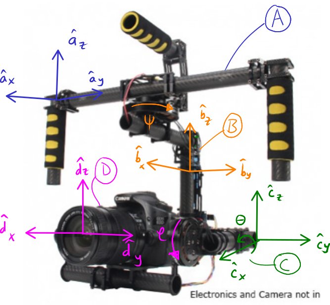
Fig. 5 Four reference frames labeled on the Turnigy Pro Steady Hand Camera Gimbal. Image copyright HobbyKing, used under fair use for educational purposes.

If we introduce two additional auxiliary reference frames, \(B\) and \(C\), attached to the intermediate camera frame members, we can use three successive simple orientations to go from \(A\) to \(D\). We can formulate the direction cosine matrices for the reference frames using the same technique for the successive simple orientations shown in Successive Orientations, but now our sequence of three orientations will enable us to orient \(D\) in any way possible relative to \(A\) in three dimensional space.

Watch this video to get a sense of the orientation axes for each intermediate auxiliary reference frame:

We first orient \(B\) with respect to \(A\) about the shared \(z\) unit vector through the angle \(\psi\), as shown below:

Fig. 6 View of the \(A\) and \(B\) \(x\textrm{-}y\) plane showing the orientation of \(B\) relative to \(A\) about \(z\) through angle \(\psi\).

In SymPy, use ReferenceFrame to establish the relative orientation:

psi = sm.symbols('psi')

A = me.ReferenceFrame('A')
B = me.ReferenceFrame('B')

B.orient_axis(A, psi, A.z)

B.dcm(A)

\[\begin{split}\displaystyle \left[\begin{matrix}\cos{\left(\psi \right)} & \sin{\left(\psi \right)} & 0\\- \sin{\left(\psi \right)} & \cos{\left(\psi \right)} & 0\\0 & 0 & 1\end{matrix}\right]\end{split}\]

Now orient \(C\) with respect to \(B\) about their shared \(x\) unit vector through angle \(\theta\).

Fig. 7 View of the \(B\) and \(C\) \(y\textrm{-}z\) plane showing the orientation of \(C\) relative to \(B\) about \(x\) through angle \(\theta\).

theta = sm.symbols('theta')

C = me.ReferenceFrame('C')

C.orient_axis(B, theta, B.x)

C.dcm(B)

\[\begin{split}\displaystyle \left[\begin{matrix}1 & 0 & 0\\0 & \cos{\left(\theta \right)} & \sin{\left(\theta \right)}\\0 & - \sin{\left(\theta \right)} & \cos{\left(\theta \right)}\end{matrix}\right]\end{split}\]

Finally, orient the camera \(D\) with respect to \(C\) about their shared \(y\) unit vector through the angle \(\phi\).

Fig. 8 View of the \(C\) and \(D\) \(x\textrm{-}z\) plane showing the orientation of \(D\) relative to \(C\) about \(y\) through angle \(\varphi\).

phi = sm.symbols('varphi')

D = me.ReferenceFrame('D')

D.orient_axis(C, phi, C.y)

D.dcm(C)

\[\begin{split}\displaystyle \left[\begin{matrix}\cos{\left(\varphi \right)} & 0 & - \sin{\left(\varphi \right)}\\0 & 1 & 0\\\sin{\left(\varphi \right)} & 0 & \cos{\left(\varphi \right)}\end{matrix}\right]\end{split}\]

With all of the intermediate orientations defined, when can now ask for the relationship \({}^D\mathbf{C}^A\) of the camera \(D\) relative to the handgrip frame \(A\):

D.dcm(A)

\[\begin{split}\displaystyle \left[\begin{matrix}- \sin{\left(\psi \right)} \sin{\left(\theta \right)} \sin{\left(\varphi \right)} + \cos{\left(\psi \right)} \cos{\left(\varphi \right)} & \sin{\left(\psi \right)} \cos{\left(\varphi \right)} + \sin{\left(\theta \right)} \sin{\left(\varphi \right)} \cos{\left(\psi \right)} & - \sin{\left(\varphi \right)} \cos{\left(\theta \right)}\\- \sin{\left(\psi \right)} \cos{\left(\theta \right)} & \cos{\left(\psi \right)} \cos{\left(\theta \right)} & \sin{\left(\theta \right)}\\\sin{\left(\psi \right)} \sin{\left(\theta \right)} \cos{\left(\varphi \right)} + \sin{\left(\varphi \right)} \cos{\left(\psi \right)} & \sin{\left(\psi \right)} \sin{\left(\varphi \right)} - \sin{\left(\theta \right)} \cos{\left(\psi \right)} \cos{\left(\varphi \right)} & \cos{\left(\theta \right)} \cos{\left(\varphi \right)}\end{matrix}\right]\end{split}\]

With these three successive orientations the camera can be rotated arbitrarily relative to the handgrip frame. These successive \(z\textrm{-}x\textrm{-}y\) orientations are a standard way of describing the orientation of two reference frames and are referred to as Euler Angles [1].

There are 12 valid sets of successive orientations that can arbitrarily orient one reference frame with respect to another. These are the six “Proper Euler Angles”:

(29)\[z\textrm{-}x\textrm{-}z, x\textrm{-}y\textrm{-}x, y\textrm{-}z\textrm{-}y, z\textrm{-}y\textrm{-}z, x\textrm{-}z\textrm{-}x, y\textrm{-}x\textrm{-}y\]

and the six “Tait-Bryan Angles”:

(30)\[x\textrm{-}y\textrm{-}z, y\textrm{-}z\textrm{-}x, z\textrm{-}x\textrm{-}y, x\textrm{-}z\textrm{-}y, z\textrm{-}y\textrm{-}x, y\textrm{-}x\textrm{-}z\]

Different sets can be more or less suitable for the kinematic nature of the system you are describing. We will also refer to these 12 possible orientation sets as “body fixed orientations”. As we will soon see, a rigid body and a reference frame are synonymous from an orientation perspective and each successive orientation rotates about a shared unit vector fixed in both of the reference frames (or bodies), thus “body fixed orientations”. The method orient_body_fixed() can be used to establish the relationship between \(A\) and \(D\) without the need to create auxiliary reference frames \(B\) and \(C\):

A = me.ReferenceFrame('A')
D = me.ReferenceFrame('D')

D.orient_body_fixed(A, (psi, theta, phi), 'zxy')

D.dcm(A)

\[\begin{split}\displaystyle \left[\begin{matrix}- \sin{\left(\psi \right)} \sin{\left(\theta \right)} \sin{\left(\varphi \right)} + \cos{\left(\psi \right)} \cos{\left(\varphi \right)} & \sin{\left(\psi \right)} \cos{\left(\varphi \right)} + \sin{\left(\theta \right)} \sin{\left(\varphi \right)} \cos{\left(\psi \right)} & - \sin{\left(\varphi \right)} \cos{\left(\theta \right)}\\- \sin{\left(\psi \right)} \cos{\left(\theta \right)} & \cos{\left(\psi \right)} \cos{\left(\theta \right)} & \sin{\left(\theta \right)}\\\sin{\left(\psi \right)} \sin{\left(\theta \right)} \cos{\left(\varphi \right)} + \sin{\left(\varphi \right)} \cos{\left(\psi \right)} & \sin{\left(\psi \right)} \sin{\left(\varphi \right)} - \sin{\left(\theta \right)} \cos{\left(\psi \right)} \cos{\left(\varphi \right)} & \cos{\left(\theta \right)} \cos{\left(\varphi \right)}\end{matrix}\right]\end{split}\]

Exercise

Euler discovered 6 of the 12 orientation sets. One of these sets is shown in this figure:

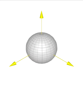
Fig. 9 An orientation through Euler angles with frame \(A\) (yellow), \(B\) (red), \(C\) (green), and \(D\) (blue). The rightward yellow arrow is the \(x\) direction, leftward yellow arrow is the \(y\) direction, and upward yellow arrow is the \(z\) direction. All frames’ unit vectors are aligned before being oriented.

Take the acute angles between \(A\) and \(B\) to be \(\psi\), \(B\) and \(C\) to be \(\theta\), and \(C\) and \(D\) to be \(\varphi\). Determine what Euler angle set this is and then calculate \({}^D\mathbf{C}^A\) using orient_axis() and then with orient_body_fixed() showing that you get the same result.

Solution

The Euler angle set is \(z\textrm{-}x\textrm{-}z\).

psi, theta, phi = sm.symbols('psi, theta, varphi')

With orient_axis():

A = me.ReferenceFrame('A')
B = me.ReferenceFrame('B')
C = me.ReferenceFrame('C')
D = me.ReferenceFrame('D')

B.orient_axis(A, psi, A.z)
C.orient_axis(B, theta, B.x)
D.orient_axis(C, phi, C.z)

D.dcm(A)

\[\begin{split}\displaystyle \left[\begin{matrix}- \sin{\left(\psi \right)} \sin{\left(\varphi \right)} \cos{\left(\theta \right)} + \cos{\left(\psi \right)} \cos{\left(\varphi \right)} & \sin{\left(\psi \right)} \cos{\left(\varphi \right)} + \sin{\left(\varphi \right)} \cos{\left(\psi \right)} \cos{\left(\theta \right)} & \sin{\left(\theta \right)} \sin{\left(\varphi \right)}\\- \sin{\left(\psi \right)} \cos{\left(\theta \right)} \cos{\left(\varphi \right)} - \sin{\left(\varphi \right)} \cos{\left(\psi \right)} & - \sin{\left(\psi \right)} \sin{\left(\varphi \right)} + \cos{\left(\psi \right)} \cos{\left(\theta \right)} \cos{\left(\varphi \right)} & \sin{\left(\theta \right)} \cos{\left(\varphi \right)}\\\sin{\left(\psi \right)} \sin{\left(\theta \right)} & - \sin{\left(\theta \right)} \cos{\left(\psi \right)} & \cos{\left(\theta \right)}\end{matrix}\right]\end{split}\]

With orient_body_fixed():

A = me.ReferenceFrame('A')
D = me.ReferenceFrame('D')

D.orient_body_fixed(A, (psi, theta, phi), 'zxz')

D.dcm(A)

\[\begin{split}\displaystyle \left[\begin{matrix}- \sin{\left(\psi \right)} \sin{\left(\varphi \right)} \cos{\left(\theta \right)} + \cos{\left(\psi \right)} \cos{\left(\varphi \right)} & \sin{\left(\psi \right)} \cos{\left(\varphi \right)} + \sin{\left(\varphi \right)} \cos{\left(\psi \right)} \cos{\left(\theta \right)} & \sin{\left(\theta \right)} \sin{\left(\varphi \right)}\\- \sin{\left(\psi \right)} \cos{\left(\theta \right)} \cos{\left(\varphi \right)} - \sin{\left(\varphi \right)} \cos{\left(\psi \right)} & - \sin{\left(\psi \right)} \sin{\left(\varphi \right)} + \cos{\left(\psi \right)} \cos{\left(\theta \right)} \cos{\left(\varphi \right)} & \sin{\left(\theta \right)} \cos{\left(\varphi \right)}\\\sin{\left(\psi \right)} \sin{\left(\theta \right)} & - \sin{\left(\theta \right)} \cos{\left(\psi \right)} & \cos{\left(\theta \right)}\end{matrix}\right]\end{split}\]

Alternatives for Representing Orientation

In the previous section, Euler-angles were used to encode the orientation of a frame or body. There are many alternative approaches to representing orientations. Three such representations, which will be used throughout this book, were already introduced:

• Euler-angles themselves, which provides a minimal representation (only 3 numbers), and a relatively straightforward way to compute the change in orientation from the angular velocity (see Angular Kinematics).

• the direction cosine matrix, which allow easy rotations or vectors and consecutive rotations, both via matrix multiplication,

• the axis-angle representation (used in the orient_axis() method), which is often an intuitive way to describe the orientation for manual input, and is useful when the axis of rotation is fixed.

Each representation also has downsides. For example, the direction cosine matrix consists of nine elements; more to keep track of than three Euler angles. Furthermore, not all combinations of nine elements form a valid direction cosine matrix, so we have to be careful to check and enforce validity when writing code.

Learn more

One more frequently used approach to representing orientations is based on so called quaternions. Quaternions are like imaginary numbers, but with three imaginary constants: \(i\), \(j\) and \(k\). These act as described by the rule

(31)\[i^2 = j^2 = k^2 = ijk = -1.\]

A general quaternion \(q\) can thus be written in terms of its components \(q_0\), \(q_i\) \(q_j\), \(q_k\) which are real numbers:

(32)\[q = q_0 + q_ii + q_jj + q_kk\]

The orient_quaternion() method enables orienting a reference frame using a quaternion in sympy:

N = me.ReferenceFrame('N')
A = me.ReferenceFrame('A')

q_0, qi, qj, qk = sm.symbols('q_0 q_i q_j q_k')
q = (q_0, qi, qj, qk)
A.orient_quaternion(N, q)
A.dcm(N)

\[\begin{split}\displaystyle \left[\begin{matrix}q_{0}^{2} + q_{i}^{2} - q_{j}^{2} - q_{k}^{2} & 2 q_{0} q_{k} + 2 q_{i} q_{j} & - 2 q_{0} q_{j} + 2 q_{i} q_{k}\\- 2 q_{0} q_{k} + 2 q_{i} q_{j} & q_{0}^{2} - q_{i}^{2} + q_{j}^{2} - q_{k}^{2} & 2 q_{0} q_{i} + 2 q_{j} q_{k}\\2 q_{0} q_{j} + 2 q_{i} q_{k} & - 2 q_{0} q_{i} + 2 q_{j} q_{k} & q_{0}^{2} - q_{i}^{2} - q_{j}^{2} + q_{k}^{2}\end{matrix}\right]\end{split}\]

A rotation of an angle \(\theta\) around a unit vector \(\hat{e}\) can be converted to a quaternion representation by having \(q_0 = \cos\left(\frac{\theta}{2}\right)\), and the other components equal to a factor \(\sin\left(\frac{\theta}{2}\right)\) times the components of the axis of rotation \(\hat{e}\). For example, if the rotation axis is \(\hat{n}_x\), we get:

q = (sm.cos(theta/2), sm.sin(theta/2), 0, 0)
A.orient_quaternion(N, q)
sm.trigsimp(A.dcm(N))

\[\begin{split}\displaystyle \left[\begin{matrix}1 & 0 & 0\\0 & \cos{\left(\theta \right)} & \sin{\left(\theta \right)}\\0 & - \sin{\left(\theta \right)} & \cos{\left(\theta \right)}\end{matrix}\right]\end{split}\]

The length of a quaternion is the square root of the sum of the squares of its components. For a quaternion representing an orientation, this length must always be 1.

It turns out that the multiplication rules for (unit) quaternions provide an efficient way to compose multiple rotations, and to numerically integrate the orientation when given an angular velocity. Due to the interpretation related to the angle and axis representation, it is also a somewhat intuitive representation. However, the integration algorithm needs to take an additional step to ensure the quaternion always has unit length.

The representation of orientations in general, turns out to be related to an area of mathematics called Lie-groups. The theory of Lie-groups has further applications to the mechanics and control of multibody systems. An example application is finding a general method for simplifying the equations for symmetric systems, so this can be done more easily and to more systems. The Lie-group theory is not used in this book. Instead, the interested reader can look up the 3D rotation group as a starting point for further study.

Footnotes

[1]

Technically, this set of angles for the gimbal are one of the 6 Tait-Bryan angles, but “Euler Angles” is used as a general term to describe both Tait-Bryan angles and “proper Euler angles”.