Mass Distribution

Note

You can download this example as a Python script: mass.py or Jupyter Notebook: mass.ipynb.

Learning Objectives

After completing this chapter readers will be able to:

• calculate the mass, mass center, and inertia of a set of particles

• use inertia vectors to find inertia scalars of a set of particles

• formulate an inertia matrix for a set of particles

• use a dyadic to manipulate 2nd order tensors in multiple reference frames

• calculate the inertia dyadic of a set of particles

• apply the parallel axis theorem

• calculate the principal moments of inertia and the principal axes

• calculate angular momentum of a rigid body

import sympy as sm
import sympy.physics.mechanics as me
me.init_vprinting(use_latex='mathjax')

class ReferenceFrame(me.ReferenceFrame):

    def __init__(self, *args, **kwargs):

        kwargs.pop('latexs', None)

        lab = args[0].lower()
        tex = r'\hat{{{}}}_{}'

        super(ReferenceFrame, self).__init__(*args,
                                             latexs=(tex.format(lab, 'x'),
                                                     tex.format(lab, 'y'),
                                                     tex.format(lab, 'z')),
                                             **kwargs)
me.ReferenceFrame = ReferenceFrame

In the prior chapters, we have developed the tools to formulate the kinematics of points and reference frames. The kinematics are the first of three essential parts needed to form the equations of motion of a multibody system; the other two being the mass distribution of and the forces acting on the system.

When a point is associated with a particle of mass \(m\) or a reference frame is associated with a rigid body that has some mass distribution, Newton’s and Euler’s second laws of motion show that the time rate of change of the linear and angular momenta must be equal to the forces and torques acting on the particle or rigid body, respectively. The momentum of a particle is determined by its mass and velocity and the angular momentum of a rigid body is determined by the distribution of mass and its angular velocity. In this chapter, we will introduce mass and its distribution.

Particles and Rigid Bodies

We will introduce and use the concepts of particles and rigid bodies in this chapter. Both are abstractions of real translating and rotating objects. Particles are points that have a location in Euclidean space which have a volumetrically infinitesimal mass. Rigid bodies are reference frames that have orientation which have an associated continuous distribution of mass. The distribution of mass can be thought of as an infinite collection of points distributed in a finite volumetric boundary. All of the points distributed in the volume are fixed to one another and translate together.

For example, an airplane can be modeled as a rigid body when one is concerned with both its translation and orientation. This could be useful when investigating its minimum turn radii and banking angle. But it could also be modeled as a particle when one is only concerned with its translation; for example when you observing the motion of the airplane from a location outside the Earth’s atmosphere.

Mass

Given a set of \(\nu\) particles with masses \(m_1,\ldots,m_\nu\) the total mass, or zeroth moment of mass, of the set is defined as:

(124)\[m := \sum_{i=1}^\nu m_i\]

Exercise

What is the mass of an object made up of two particles of mass \(m\) and a rigid body with mass \(m/2\)?

Solution

m = sm.symbols('m')

m_total = m + m + m/2
m_total

\[\displaystyle \frac{5 m}{2}\]

For a rigid body consisting of a solid with a density \(\rho\) defined at each point within its volumetric \(V\) boundary, the total mass becomes an integral of the general form:

(125)\[m := \int_{\textrm{solid}} \rho dV\]

Exercise

What is the mass of a cone with uniform density \(\rho\), radius \(R\), and height \(h\)?

Solution

Using cylindrical coordinates to write \(dV=r \mathrm{d}z \mathrm{d}\theta \mathrm{d}r\), integrate() function can solve the triple integral:

(126)\[\int_0^h \int_0^{2\pi} \int_0^{\frac{R}{h}z} \rho r \mathrm{d}{z} \mathrm{d}{\theta} \mathrm{d}r\]

p, R, h = sm.symbols('rho, R, h')  # constants
r, z, theta = sm.symbols('r, z, theta')  # integration variables

sm.integrate(p*r, (r, 0, R/h*z), (theta, 0, 2*sm.pi), (z, 0, h))

\[\displaystyle \frac{\pi R^{2} h \rho}{3}\]

Mass Center

If each particle in a set of \(S\) particles is located at positions \(\bar{r}^{P_i/O},\ldots,\bar{r}^{P_\nu/O}\) the first moment of mass is defined as:

(127)\[\sum_{i=1}^\nu m_i \bar{r}^{P_i/O}\textrm{.}\]

There is then a point \(S_o\) in which the first mass moment is equal to zero; fulfilling the following equation:

(128)\[\sum_{i=1}^\nu m_i \bar{r}^{P_i/S_o} = 0\textrm{.}\]

This point \(S_o\) is referred to as the mass center (or center of mass) of the set of particles. The mass center’s position can be found by dividing the first moment of mass by the zeroth moment of mass:

(129)\[\bar{r}^{S_o/O} = \frac{ \sum_{i=1}^\nu m_i \bar{r}^{P_i/O} }{\sum_{i=1}^\nu m_i}\textrm{.}\]

For a solid body, this takes the integral form:

(130)\[\bar{r}^{S_o/O} = \frac{ \int_{\textrm{solid}} \rho \bar{r} dV }{ \int_{\textrm{solid}} \rho dV }\]

The particle form (Eq. (129)) can be calculated using vectors and scalars in SymPy Mechanics. Here is an example of three particles each at an arbitrary location relative to \(O\):

m1, m2, m3 = sm.symbols('m1, m2, m3')
x1, x2, x3 = me.dynamicsymbols('x1, x2, x3')
y1, y2, y3 = me.dynamicsymbols('y1, y2, y3')
z1, z2, z3 = me.dynamicsymbols('z1, z2, z3')

A = me.ReferenceFrame('A')

zeroth_moment = (m1 + m2 + m3)

first_moment = (m1*(x1*A.x + y1*A.y + z1*A.z) +
                m2*(x2*A.x + y2*A.y + z2*A.z) +
                m3*(x3*A.x + y3*A.y + z3*A.z))
first_moment

\[\displaystyle (m_{1} x_{1} + m_{2} x_{2} + m_{3} x_{3})\hat{a}_x + (m_{1} y_{1} + m_{2} y_{2} + m_{3} y_{3})\hat{a}_y + (m_{1} z_{1} + m_{2} z_{2} + m_{3} z_{3})\hat{a}_z\]

r_O_So =  first_moment/zeroth_moment
r_O_So

\[\displaystyle \frac{m_{1} x_{1} + m_{2} x_{2} + m_{3} x_{3}}{m_{1} + m_{2} + m_{3}}\hat{a}_x + \frac{m_{1} y_{1} + m_{2} y_{2} + m_{3} y_{3}}{m_{1} + m_{2} + m_{3}}\hat{a}_y + \frac{m_{1} z_{1} + m_{2} z_{2} + m_{3} z_{3}}{m_{1} + m_{2} + m_{3}}\hat{a}_z\]

Exercise

If \(m_2=2m_1\) and \(m_3=3m_1\) in the above example, find the mass center.

Solution

r_O_So.xreplace({m2: 2*m1, m3: 3*m1}).simplify()

\[\displaystyle (\frac{x_{1}}{6} + \frac{x_{2}}{3} + \frac{x_{3}}{2})\hat{a}_x + (\frac{y_{1}}{6} + \frac{y_{2}}{3} + \frac{y_{3}}{2})\hat{a}_y + (\frac{z_{1}}{6} + \frac{z_{2}}{3} + \frac{z_{3}}{2})\hat{a}_z\]

Distribution of Mass

The inertia, or second moment of mass, describes the distribution of mass relative to a point about an axis. Inertia characterizes the resistance to angular acceleration in the same way that mass characterizes the resistance to linear acceleration. For a set of particles \(P_1,\ldots,P_\nu\) with positions \(\bar{r}^{P_1/O},\ldots,\bar{r}^{P_\nu/O}\) all relative to a point \(O\), the inertia vector about the unit vector \(\hat{n}_a\) is defined as ([Kane1985], pg. 61):

(131)\[\bar{I}_a := \sum_{i=1}^\nu m_i \bar{r}^{P_i/O} \times \left( \hat{n}_a \times \bar{r}^{P_i/O} \right)\]

Similarly, for an infinite number of points at locations parametrized by \(\tau\) that make up a rigid body with density \(\rho(\tau)\) the integral form is used ([Kane1985], pg. 62):

(132)\[\bar{I}_a := \int_{\textrm{solid}} \rho(\tau) \left[ \bar{r}^{P(\tau)/O} \times \left( \hat{n}_a \times \bar{r}^{P(\tau)/O} \right) \right] d\tau\]

This vector describes the sum of each mass’s contribution to the mass distribution about a line that is parallel to \(\hat{n}_a\) and passes through \(O\). Figure Fig. 32 shows a visual representation of this vector for a single particle \(P\) with mass \(m\).

Fig. 32 Inertia vector for a single particle \(P\) of mass \(m\) and its relationship to \(\hat{n}_a\).

For this single particle, the magnitude of \(\bar{I}_a\) is:

(133)\[\left| \bar{I}_a \right| = m \left| \bar{r}^{P/O} \right| ^2 | \sin\theta |\]

where \(\theta\) is angle between \(\bar{r}^{P/O}\) and \(\hat{n}_a\). We see that \(\bar{I}_a\) is always perpendicular to \(\bar{r}^{P/O}\) and scales with \(m\), \(| \bar{r}^{P/O} |^2\), and \(\sin\theta\). If \(\hat{n}_a\) happens to be parallel to \(\bar{r}^{P/O}\) then the magnitude of \(\bar{I}_a\) is zero. If \(\hat{n}_a\) is perpendicular to \(\bar{r}^{P/O}\) then the magnitude is:

(134)\[\left| \bar{I}_a \right| = m \left| \bar{r}^{P/O} \right| ^2\]

The inertia vector fully describes the distribution of the particles with respect to \(O\) about \(\hat{n}_a\).

A component of \(\bar{I}_a\) in the \(\hat{n}_b\) direction is called an inertia scalar and is defined as ([Kane1985], pg. 62):

(135)\[I_{ab} := \bar{I}_{a} \cdot \hat{n}_b\]

The inertia scalar can be rewritten using Eq. (131) as:

(136)\[I_{ab} = \sum_{i=1}^\nu m_i \left( \bar{r}^{P_i/O} \times \hat{n}_a \right) \cdot \left( \bar{r}^{P_i/O} \times \hat{n}_b \right)\textrm{.}\]

This form implies that:

(137)\[I_{ab} = I_{ba}\]

If \(\hat{n}_a = \hat{n}_b\) then this inertia scalar is called a moment of inertia and if \(\hat{n}_a \neq \hat{n}_b\) it is called a product of inertia. Moments of inertia describe the mass distribution about a single axis whereas products of inertia describe the mass distribution relative to two axes.

When \(\hat{n}_a = \hat{n}_b\) Eq. (136) reduces to the moment of inertia:

(138)\[I_{aa} = \sum_{i=1}^\nu m_i \left( \bar{r}^{P_i/O} \times \hat{n}_a \right) \cdot \left( \bar{r}^{P_i/O} \times \hat{n}_a \right)\]

It is common to define the radius of gyration \(k_{aa}\), which is the radius of a ring that has the same moment of inertia as the set of particles or rigid body. The radius of gyration about a line through \(O\) parallel to \(\hat{n}_a\) is defined as:

(139)\[k_{aa} := \sqrt{\frac{I_{aa}}{m}}\]

Exercise

Three masses of \(m\), \(2m\), and \(3m\) slide on a ring of radius \(r\). Mass \(3m\) always lies \(\pi/6\) anitclockwise from \(m\) and mass \(2m\) always lies \(\pi/7\) clockwise from \(m\). Find the acute angle from the line from the ring center to \(m\) to a line tangent to the ring at point \(O\) which minimizes the total radius of gyration of all three masses about the line tangent to the ring.

Solution

Define the necessary variables, including \(\theta\) to locate mass \(m\).

m, r, theta = sm.symbols('m, r, theta')
A = me.ReferenceFrame('A')

Create position vectors to each of the masses:

r_O_m = (r + r*sm.sin(theta))*A.x + r*sm.cos(theta)*A.y
r_O_2m = (r + r*sm.sin(theta + sm.pi/7))*A.x + r*sm.cos(theta + sm.pi/7)*A.y
r_O_3m = (r + r*sm.sin(theta - sm.pi/6))*A.x + r*sm.cos(theta - sm.pi/6)*A.y

Create the inertia scalar for a moment of inertia about the point \(O\) and \(\hat{a}_y\).

Iyy = (m*me.dot(r_O_m.cross(A.y), r_O_m.cross(A.y)) +
       2*m*me.dot(r_O_2m.cross(A.y), r_O_2m.cross(A.y)) +
       3*m*me.dot(r_O_3m.cross(A.y), r_O_3m.cross(A.y)))
Iyy

\[\displaystyle m \left(r \sin{\left(\theta \right)} + r\right)^{2} + 2 m \left(r \sin{\left(\theta + \frac{\pi}{7} \right)} + r\right)^{2} + 3 m \left(- r \cos{\left(\theta + \frac{\pi}{3} \right)} + r\right)^{2}\]

Recognizing that the radius of gyration is minimized when the moment of inertia is minimized, we can take the derivative of the moment of inertia with respect to \(\theta\) and set that equal to zero.

dIyydtheta = sm.simplify(Iyy.diff(theta))
dIyydtheta

\[\displaystyle 2 m r^{2} \left(\left(\sin{\left(\theta \right)} + 1\right) \cos{\left(\theta \right)} + 2 \left(\sin{\left(\theta + \frac{\pi}{7} \right)} + 1\right) \cos{\left(\theta + \frac{\pi}{7} \right)} - 3 \left(\cos{\left(\theta + \frac{\pi}{3} \right)} - 1\right) \sin{\left(\theta + \frac{\pi}{3} \right)}\right)\]

We can divide through by \(mr^2\) and solve numerically for \(\theta\) since it is the only variable present in the expression.

theta_sol = sm.nsolve((dIyydtheta/m/r**2).evalf(), theta, 0)
theta_sol

\[\displaystyle -1.49935061382135\]

In degrees that is:

import math

theta_sol*180/math.pi

\[\displaystyle -85.9064621823125\]

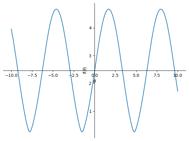
The plot() function can make quick plots of single variate functions. Here we see that rotating the set of masses around the ring will maximize and minimize the radius of gyration and that our solution is a minima. \(m=r=1\) was selected so we could plot only as a function of \(\theta\).

kyy = sm.sqrt(Iyy/m)
kyy

\[\displaystyle \sqrt{\frac{m \left(r \sin{\left(\theta \right)} + r\right)^{2} + 2 m \left(r \sin{\left(\theta + \frac{\pi}{7} \right)} + r\right)^{2} + 3 m \left(- r \cos{\left(\theta + \frac{\pi}{3} \right)} + r\right)^{2}}{m}}\]

sm.plot(kyy.xreplace({m: 1, r: 1}));

kyy.xreplace({m: 1, r: 1, theta: theta_sol}).evalf()

\[\displaystyle 0.255558185585985\]

Inertia Matrix

For mutually perpendicular unit vectors fixed in reference frame \(A\), the moments of inertia with respect to \(O\) about each unit vector and the products of inertia among the pairs of perpendicular unit vectors can be computed using the inertia vector expressions in the prior section. This, in general, results in nine inertia scalars (6 unique scalars because of (137)) that describe the mass distribution of a set of particles or a rigid body in 3D space. These scalars are typically presented as a symmetric inertia matrix (also called an inertia tensor) that takes this form:

(140)\[\begin{split}\begin{bmatrix} I_{xx} & I_{xy} & I_{xz} \\ I_{yx} & I_{yy} & I_{yz} \\ I_{zx} & I_{zy} & I_{zz} \end{bmatrix}_A\end{split}\]

where the moments of inertia are on the diagonal and the products of inertia are the off diagonal entries. Eq. (137) holds for the products of inertia, i.e. \(I_{xy}=I_{yx}\), \(I_{xz}=I_{zx}\), and \(I_{yz}=I_{zy}\), and the subscript \(A\) indicates that these scalars are relative to mutually perpendicular unit vectors \(\hat{a}_x,\hat{a}_y,\hat{a}_z\) fixed in \(A\).

This matrix (or second order tensor) is similar to the vectors (or first order tensors) we’ve already worked with:

(141)\[\begin{split}\begin{bmatrix} v_1 \\ v_2 \\ v_3 \end{bmatrix}_A\end{split}\]

Recall that we have a notation for writing such a vector that allows us to combine components expressed in different reference frames:

(142)\[v_1\hat{a}_x + v_2\hat{a}_y + v_3\hat{a}_z\]

There also exists an analogous form for second order tensors that are associated with different reference frames called a dyadic.

Dyadics

If we introduce the outer product operator between two vectors we see that it generates a matrix akin to the inertia matrix above.

(143)\[\begin{split}\begin{bmatrix} v_1 \\ v_2 \\ v_3 \end{bmatrix}_A \otimes \begin{bmatrix} w_1 \\ w_2 \\ w_3 \end{bmatrix}_A = \begin{bmatrix} v_1w_1 & v_1w_2 & v_1w_3 \\ v_2w_1 & v_2w_2 & v_2w_3 \\ v_3w_1 & v_3w_2 & v_3w_3 \\ \end{bmatrix}_A\end{split}\]

In SymPy Mechanics, outer products can be taken between two vectors to create the dyadic \(\breve{Q}\) using outer():

v1, v2, v3 = sm.symbols('v1, v2, v3')
w1, w2, w3 = sm.symbols('w1, w2, w3')

A = me.ReferenceFrame('A')

v = v1*A.x + v2*A.y + v3*A.z
w = w1*A.x + w2*A.y + w3*A.z

Q = me.outer(v, w)
Q

\[\displaystyle v_{1} w_{1}\hat{a}_x\otimes \hat{a}_x + v_{1} w_{2}\hat{a}_x\otimes \hat{a}_y + v_{1} w_{3}\hat{a}_x\otimes \hat{a}_z + v_{2} w_{1}\hat{a}_y\otimes \hat{a}_x + v_{2} w_{2}\hat{a}_y\otimes \hat{a}_y + v_{2} w_{3}\hat{a}_y\otimes \hat{a}_z + v_{3} w_{1}\hat{a}_z\otimes \hat{a}_x + v_{3} w_{2}\hat{a}_z\otimes \hat{a}_y + v_{3} w_{3}\hat{a}_z\otimes \hat{a}_z\]

The result is not the matrix form shown in Eq. (143), but instead the result is a dyadic. The dyadic is the analogous form for second order tensors to what we have been using for first order tensors, i.e. vectors. If the matrix form is needed, it can be found with to_matrix() and naming a specific reference frame to express the dyadic in:

Q.to_matrix(A)

\[\begin{split}\displaystyle \left[\begin{matrix}v_{1} w_{1} & v_{1} w_{2} & v_{1} w_{3}\\v_{2} w_{1} & v_{2} w_{2} & v_{2} w_{3}\\v_{3} w_{1} & v_{3} w_{2} & v_{3} w_{3}\end{matrix}\right]\end{split}\]

The dyadic is made up of scalars multiplied by unit dyads. Examples of unit dyads are:

me.outer(A.x, A.x)

\[\displaystyle \hat{a}_x\otimes \hat{a}_x\]

Unit dyads correspond to unit entries in the 3x3 matrix:

me.outer(A.x, A.x).to_matrix(A)

\[\begin{split}\displaystyle \left[\begin{matrix}1 & 0 & 0\\0 & 0 & 0\\0 & 0 & 0\end{matrix}\right]\end{split}\]

Unit dyads are analogous to unit vectors. There are nine unit dyads in total associated with the three orthogonal unit vectors. Here is another example:

me.outer(A.y, A.z)

\[\displaystyle \hat{a}_y\otimes \hat{a}_z\]

me.outer(A.y, A.z).to_matrix(A)

\[\begin{split}\displaystyle \left[\begin{matrix}0 & 0 & 0\\0 & 0 & 1\\0 & 0 & 0\end{matrix}\right]\end{split}\]

These unit dyads can be formed from any unit vectors. This is convenient because we can create dyadics, just like vectors, which are made up of components in different reference frames. For example:

theta = sm.symbols("theta")

A = me.ReferenceFrame('A')
B = me.ReferenceFrame('B')

B.orient_axis(A, theta, A.x)

P = 2*me.outer(B.x, B.x) + 3*me.outer(A.x, B.y) + 4*me.outer(B.z, A.z)
P

\[\displaystyle 2\hat{b}_x\otimes \hat{b}_x + 3\hat{a}_x\otimes \hat{b}_y + 4\hat{b}_z\otimes \hat{a}_z\]

The dyadic \(\breve{P}\) can be expressed in unit dyads of \(A\)

P.express(A)

\[\displaystyle 2\hat{a}_x\otimes \hat{a}_x + 3 \cos{\left(\theta \right)}\hat{a}_x\otimes \hat{a}_y + 3 \sin{\left(\theta \right)}\hat{a}_x\otimes \hat{a}_z - 4 \sin{\left(\theta \right)}\hat{a}_y\otimes \hat{a}_z + 4 \cos{\left(\theta \right)}\hat{a}_z\otimes \hat{a}_z\]

P.to_matrix(A)

\[\begin{split}\displaystyle \left[\begin{matrix}2 & 3 \cos{\left(\theta \right)} & 3 \sin{\left(\theta \right)}\\0 & 0 & - 4 \sin{\left(\theta \right)}\\0 & 0 & 4 \cos{\left(\theta \right)}\end{matrix}\right]\end{split}\]

or \(B\): :

P.express(B)

\[\displaystyle 2\hat{b}_x\otimes \hat{b}_x + 3\hat{b}_x\otimes \hat{b}_y + 4 \sin{\left(\theta \right)}\hat{b}_z\otimes \hat{b}_y + 4 \cos{\left(\theta \right)}\hat{b}_z\otimes \hat{b}_z\]

P.to_matrix(B)

\[\begin{split}\displaystyle \left[\begin{matrix}2 & 3 & 0\\0 & 0 & 0\\0 & 4 \sin{\left(\theta \right)} & 4 \cos{\left(\theta \right)}\end{matrix}\right]\end{split}\]

The unit dyadic is defined as:

(144)\[\breve{U} := \hat{a}_x \otimes \hat{a}_x + \hat{a}_y \otimes \hat{a}_y + \hat{a}_z \otimes \hat{a}_z\]

The unit dyadic can be created with SymPy:

U = me.outer(A.x, A.x) + me.outer(A.y, A.y) + me.outer(A.z, A.z)
U

\[\displaystyle \hat{a}_x\otimes \hat{a}_x + \hat{a}_y\otimes \hat{a}_y + \hat{a}_z\otimes \hat{a}_z\]

and it represents the identity matrix in \(A\):

U.to_matrix(A)

\[\begin{split}\displaystyle \left[\begin{matrix}1 & 0 & 0\\0 & 1 & 0\\0 & 0 & 1\end{matrix}\right]\end{split}\]

Note that the unit dyadic is the same when expressed in any reference frame:

U.express(B).simplify()

\[\displaystyle \hat{b}_x\otimes \hat{b}_x + \hat{b}_y\otimes \hat{b}_y + \hat{b}_z\otimes \hat{b}_z\]

Properties of Dyadics

Dyadics have similar properties as vectors but are not necessarily commutative.

• Scalar multiplication: \(\alpha(\bar{u}\otimes\bar{v}) = \alpha\bar{u}\otimes\bar{v} = \bar{u}\otimes\alpha\bar{v}\)

• Distributive: \(\bar{u}\otimes(\bar{v} + \bar{w}) = \bar{u}\otimes\bar{v} + \bar{u}\otimes\bar{w}\)

• Left and right dot product with a vector (results in a vector):

  • \(\bar{u}\cdot(\bar{v}\otimes\bar{w}) = (\bar{u}\cdot\bar{v})\bar{w}\)

  • \((\bar{u}\otimes\bar{v})\cdot\bar{w} = \bar{u}(\bar{v}\cdot\bar{w})\)

• Left and right cross product with a vector (results in a dyadic):

  • \(\bar{u}\times(\bar{v}\otimes\bar{w}) = (\bar{u}\times\bar{v})\otimes\bar{w}\)

  • \((\bar{u}\otimes\bar{v})\times\bar{w} = \bar{u}\otimes(\bar{v}\times\bar{w})\)

• Dot products between arbitrary vectors \(\bar{u}\) and arbitrary dyadics \(\breve{V}\) are not commutative: \(\breve{V}\cdot\bar{u} \neq \bar{u}\cdot\breve{V}\)

• Dot products between arbitrary vectors and the unit dyadic are commutative and result in the vector itself: \(\breve{U}\cdot\bar{v} = \bar{v}\cdot\breve{U} = \bar{v}\)

Inertia Dyadic

Previously we defined the inertia vector for a set of \(\nu\) particles as:

(145)\[\bar{I}_a = \sum_{i=1}^\nu m_i \bar{r}^{P_i/O} \times \left( \hat{n}_a \times \bar{r}^{P_i/O} \right)\]

Using the vector triple product identity: \(\bar{a}\times(\bar{b}\times\bar{c}) = \bar{b}(\bar{a}\cdot\bar{c}) - \bar{c}(\bar{a}\cdot\bar{b})\), the inertia vector can be written as ([Kane1985], pg. 68):

(146)\[\bar{I}_a = \sum_{i=1}^\nu m_i \left[\hat{n}_a \left( \bar{r}^{P_i/O} \cdot \bar{r}^{P_i/O} \right) - \bar{r}^{P_i/O} \left( \bar{r}^{P_i/O} \cdot \hat{n}_a \right) \right]\]

Now by introducing a unit dyadic, we can write:

(147)\[\bar{I}_a = \sum_{i=1}^\nu m_i \left[ \left|\bar{r}^{P_i/O}\right|^2 \hat{n}_a \cdot \breve{U} - \hat{n}_a \cdot \left(\bar{r}^{P_i/O} \otimes \bar{r}^{P_i/O}\right) \right]\]

\(\hat{n}_a\) can be pulled out of the summation:

(148)\[\bar{I}_a = \hat{n}_a \cdot \sum_{i=1}^\nu m_i \left( \left|\bar{r}^{P_i/O}\right|^2 \breve{U} - \bar{r}^{P_i/O} \otimes \bar{r}^{P_i/O} \right)\]

The inertia dyadic \(\breve{I}\) of a set of \(S\) particles relative to \(O\) is now defined as:

(149)\[\breve{I}^{S/O} := \sum_{i=1}^\nu m_i \left( \left|\bar{r}^{P_i/O}\right|^2 \breve{U} - \bar{r}^{P_i/O} \otimes \bar{r}^{P_i/O} \right)\]

where:

(150)\[\bar{I}_a = \hat{n}_a \cdot \breve{I}^{S/O}\]

Note that we have now described the inertia of the set of particles without needing to specify a vector \(\hat{n}_a\). This inertia dyadic contains the complete description of inertia with respect to point \(O\) about any axis. The vectors and dyadics in Eq. (149) can be written in terms of any reference frame unit vectors or unit dyads, respectively.

If you have a solid body, an infinite set of points with a volumetric boundary, then you must solve the integral version of (149) where the position of any location in the particle is parameterize by \(\tau\) which can represent a volume, line, or surface parameterization.

(151)\[\breve{I}^{S/O} := \int_\textrm{solid} \rho \left( \left|\bar{r}^{P(\tau)/O}\right|^2 \breve{U} - \bar{r}^{P(\tau)/O} \otimes \bar{r}^{P(\tau)/O} \right) \textrm{d}\tau\]

In SymPy Mechanics, simple inertia dyadics in terms of the unit vectors of a single reference frame can quickly be generated with inertia(). For example:

Ixx, Iyy, Izz = sm.symbols('I_{xx}, I_{yy}, I_{zz}')
Ixy, Iyz, Ixz = sm.symbols('I_{xy}, I_{yz}, I_{xz}')

I = me.inertia(A, Ixx, Iyy, Izz, ixy=Ixy, iyz=Iyz, izx=Ixz)
I

\[\displaystyle I_{xx}\hat{a}_x\otimes \hat{a}_x + I_{xy}\hat{a}_x\otimes \hat{a}_y + I_{xz}\hat{a}_x\otimes \hat{a}_z + I_{xy}\hat{a}_y\otimes \hat{a}_x + I_{yy}\hat{a}_y\otimes \hat{a}_y + I_{yz}\hat{a}_y\otimes \hat{a}_z + I_{xz}\hat{a}_z\otimes \hat{a}_x + I_{yz}\hat{a}_z\otimes \hat{a}_y + I_{zz}\hat{a}_z\otimes \hat{a}_z\]

I.to_matrix(A)

\[\begin{split}\displaystyle \left[\begin{matrix}I_{xx} & I_{xy} & I_{xz}\\I_{xy} & I_{yy} & I_{yz}\\I_{xz} & I_{yz} & I_{zz}\end{matrix}\right]\end{split}\]

This inertia dyadic can easily be expressed relative to another reference frame if the orientation is defined (demonstrated above in Dyadics):

I.express(B).simplify()

\[\displaystyle I_{xx}\hat{b}_x\otimes \hat{b}_x + (I_{xy} \cos{\left(\theta \right)} + I_{xz} \sin{\left(\theta \right)})\hat{b}_x\otimes \hat{b}_y + (- I_{xy} \sin{\left(\theta \right)} + I_{xz} \cos{\left(\theta \right)})\hat{b}_x\otimes \hat{b}_z + (I_{xy} \cos{\left(\theta \right)} + I_{xz} \sin{\left(\theta \right)})\hat{b}_y\otimes \hat{b}_x + (- I_{xy} \sin{\left(\theta \right)} + I_{xz} \cos{\left(\theta \right)})\hat{b}_z\otimes \hat{b}_x + (I_{yy} \cos^{2}{\left(\theta \right)} + I_{yz} \sin{\left(2 \theta \right)} + I_{zz} \sin^{2}{\left(\theta \right)})\hat{b}_y\otimes \hat{b}_y + (- \frac{I_{yy} \sin{\left(2 \theta \right)}}{2} + I_{yz} \cos{\left(2 \theta \right)} + \frac{I_{zz} \sin{\left(2 \theta \right)}}{2})\hat{b}_y\otimes \hat{b}_z + (- \frac{I_{yy} \sin{\left(2 \theta \right)}}{2} + I_{yz} \cos{\left(2 \theta \right)} + \frac{I_{zz} \sin{\left(2 \theta \right)}}{2})\hat{b}_z\otimes \hat{b}_y + (I_{yy} \sin^{2}{\left(\theta \right)} - I_{yz} \sin{\left(2 \theta \right)} + I_{zz} \cos^{2}{\left(\theta \right)})\hat{b}_z\otimes \hat{b}_z\]

or as a matrix in \(B\):

I.express(B).simplify().to_matrix(B)

\[\begin{split}\displaystyle \left[\begin{matrix}I_{xx} & I_{xy} \cos{\left(\theta \right)} + I_{xz} \sin{\left(\theta \right)} & - I_{xy} \sin{\left(\theta \right)} + I_{xz} \cos{\left(\theta \right)}\\I_{xy} \cos{\left(\theta \right)} + I_{xz} \sin{\left(\theta \right)} & I_{yy} \cos^{2}{\left(\theta \right)} + I_{yz} \sin{\left(2 \theta \right)} + I_{zz} \sin^{2}{\left(\theta \right)} & - \frac{I_{yy} \sin{\left(2 \theta \right)}}{2} + I_{yz} \cos{\left(2 \theta \right)} + \frac{I_{zz} \sin{\left(2 \theta \right)}}{2}\\- I_{xy} \sin{\left(\theta \right)} + I_{xz} \cos{\left(\theta \right)} & - \frac{I_{yy} \sin{\left(2 \theta \right)}}{2} + I_{yz} \cos{\left(2 \theta \right)} + \frac{I_{zz} \sin{\left(2 \theta \right)}}{2} & I_{yy} \sin^{2}{\left(\theta \right)} - I_{yz} \sin{\left(2 \theta \right)} + I_{zz} \cos^{2}{\left(\theta \right)}\end{matrix}\right]\end{split}\]

This is equivalent to the matrix transform to express an inertia matrix in other reference frame (see some explanations on Wikipedia about this transform):

(152)\[{}^B\mathbf{C}^A \ \mathbf{I} \ {}^A\mathbf{C}^B\]

sm.simplify(B.dcm(A)*I.to_matrix(A)*A.dcm(B))

\[\begin{split}\displaystyle \left[\begin{matrix}I_{xx} & I_{xy} \cos{\left(\theta \right)} + I_{xz} \sin{\left(\theta \right)} & - I_{xy} \sin{\left(\theta \right)} + I_{xz} \cos{\left(\theta \right)}\\I_{xy} \cos{\left(\theta \right)} + I_{xz} \sin{\left(\theta \right)} & I_{yy} \cos^{2}{\left(\theta \right)} + I_{yz} \sin{\left(2 \theta \right)} + I_{zz} \sin^{2}{\left(\theta \right)} & - \frac{I_{yy} \sin{\left(2 \theta \right)}}{2} + I_{yz} \cos{\left(2 \theta \right)} + \frac{I_{zz} \sin{\left(2 \theta \right)}}{2}\\- I_{xy} \sin{\left(\theta \right)} + I_{xz} \cos{\left(\theta \right)} & - \frac{I_{yy} \sin{\left(2 \theta \right)}}{2} + I_{yz} \cos{\left(2 \theta \right)} + \frac{I_{zz} \sin{\left(2 \theta \right)}}{2} & I_{yy} \sin^{2}{\left(\theta \right)} - I_{yz} \sin{\left(2 \theta \right)} + I_{zz} \cos^{2}{\left(\theta \right)}\end{matrix}\right]\end{split}\]

Exercise

Fig. 33 Head tube angle of a bicycle.

Given the inertia dyadic of a bicycle’s handlebar and fork assembly about its mass center where \(\hat{n}_x\) points from the center of the rear wheel to the center of the front wheel and \(\hat{n}_z\) points downward, normal to the ground, and the head tube angle is 68 degrees from the ground plane, find the moment of inertia about the tilted steer axis given the inertia dyadic:

N = me.ReferenceFrame('N')

I = (0.25*me.outer(N.x, N.x) +
     0.25*me.outer(N.y, N.y) +
     0.10*me.outer(N.z, N.z) -
     0.07*me.outer(N.x, N.z) -
     0.07*me.outer(N.z, N.x))
I

\[\displaystyle 0.25\hat{n}_x\otimes \hat{n}_x + 0.25\hat{n}_y\otimes \hat{n}_y + 0.1\hat{n}_z\otimes \hat{n}_z - 0.07\hat{n}_x\otimes \hat{n}_z - 0.07\hat{n}_z\otimes \hat{n}_x\]

Solution

Create a new reference frame that has \(\hat{h}_z\) aligned with the steer axis.

H = me.ReferenceFrame('H')
H.orient_axis(N, sm.pi/2 - 68.0*sm.pi/180, N.y)

Dot the inertia dyadic twice with \(\hat{h}_z\) to get the moment of inertia about the steer axis:

I.dot(H.z).dot(H.z).evalf()

\[\displaystyle 0.0724234290424714\]

Alternatively, you can use the matrix transformation.

I.to_matrix(N)

\[\begin{split}\displaystyle \left[\begin{matrix}0.25 & 0 & -0.07\\0 & 0.25 & 0\\-0.07 & 0 & 0.1\end{matrix}\right]\end{split}\]

I_H = (H.dcm(N) @ I.to_matrix(N) @ N.dcm(H)).evalf()
I_H

\[\begin{split}\displaystyle \left[\begin{matrix}0.277576570957529 & 0 & 0.00174559176071922\\0 & 0.25 & 0\\0.00174559176071922 & 0 & 0.0724234290424714\end{matrix}\right]\end{split}\]

I_H[2, 2]

\[\displaystyle 0.0724234290424714\]

Parallel Axis Theorem

If you know the central inertia dyadic of a rigid body \(B\) (or equivalently a set of particles) about its mass center \(B_o\) then it is possible to calculate the inertia dyadic about any other point \(O\). To do so, you must account for the inertial contribution due to the distance between the points \(O\) and \(B_o\). This is done with the parallel axis theorem ([Kane1985], pg. 70):

(153)\[\breve{I}^{B/O} = \breve{I}^{B/B_o} + \breve{I}^{B_o/O}\]

The last term is the inertia of a particle with mass \(m\) (total mass of the body or set of particles) located at the mass center about point \(O\).

(154)\[\breve{I}^{B_o/O} = m \left( \left|\bar{r}^{B_o/O}\right|^2 \breve{U} - \bar{r}^{B_o/O} \otimes \bar{r}^{B_o/O} \right)\]

When \(B_o\) is displaced from point \(O\) by three Cartesian distances \(d_x,d_y,d_z\) the general form of the last term in Eq. (153) can be found:

dx, dy, dz, m = sm.symbols('d_x, d_y, d_z, m')

N = me.ReferenceFrame('N')

r_O_Bo = dx*N.x + dy*N.y + dz*N.z

U = me.outer(N.x, N.x) + me.outer(N.y, N.y) + me.outer(N.z, N.z)

I_Bo_O = m*(me.dot(r_O_Bo, r_O_Bo)*U - me.outer(r_O_Bo, r_O_Bo))
I_Bo_O

\[\displaystyle m \left(d_{y}^{2} + d_{z}^{2}\right)\hat{n}_x\otimes \hat{n}_x + m \left(d_{x}^{2} + d_{z}^{2}\right)\hat{n}_y\otimes \hat{n}_y + m \left(d_{x}^{2} + d_{y}^{2}\right)\hat{n}_z\otimes \hat{n}_z - d_{x} d_{y} m\hat{n}_x\otimes \hat{n}_y - d_{x} d_{z} m\hat{n}_x\otimes \hat{n}_z - d_{x} d_{y} m\hat{n}_y\otimes \hat{n}_x - d_{y} d_{z} m\hat{n}_y\otimes \hat{n}_z - d_{x} d_{z} m\hat{n}_z\otimes \hat{n}_x - d_{y} d_{z} m\hat{n}_z\otimes \hat{n}_y\]

The matrix form of this dyadic shows the typical presentation of the parallel axis addition term:

I_Bo_O.to_matrix(N)

\[\begin{split}\displaystyle \left[\begin{matrix}m \left(d_{y}^{2} + d_{z}^{2}\right) & - d_{x} d_{y} m & - d_{x} d_{z} m\\- d_{x} d_{y} m & m \left(d_{x}^{2} + d_{z}^{2}\right) & - d_{y} d_{z} m\\- d_{x} d_{z} m & - d_{y} d_{z} m & m \left(d_{x}^{2} + d_{y}^{2}\right)\end{matrix}\right]\end{split}\]

Principal Axes and Moments of Inertia

If the inertia vector \(\bar{I}_a\) with respect to point \(O\) is parallel to its unit vector \(\hat{n}_a\) then the line through \(O\) and parallel to \(\hat{n}_a\) is called a principal axis of the set of particles or rigid body. The plane that is normal to \(\hat{n}_a\) is called a principal plane. The moment of inertia about this principal axis is called a principal moment of inertia. The consequence of \(\bar{I}_a\) being parallel to \(\hat{n}_a\) is that the products of inertia are all zero. The principal inertia dyadic can then be written as so:

(155)\[\breve{I}^{B/O} = I_{11} \hat{b}_1 \otimes \hat{b}_1 + I_{22} \hat{b}_2 \otimes \hat{b}_2 + I_{33} \hat{b}_3 \otimes \hat{b}_3\]

where \(\hat{b}_1,\hat{b}_2,\hat{b}_3\) are mutually perpendicular unit vectors in \(B\) that are each parallel to a principal axis and \(I_{11},I_{22},I_{33}\) are all principal moments of inertia.

Geometrically symmetric objects with uniform mass density have principal planes that are perpendicular with the planes of symmetry of the geometry. But it is important to note that there also exist unique principal axes for all non-symmetric and non-uniform density objects, i.e. having geometric symmetry is not necessary to have principal moments of inertia; all rigid bodies have principal moments of inertia and associated axes.

The principal axes and their associated principal moments of inertia can be found by solving the eigenvalue problem. The eigenvalues of an arbitrary inertia matrix are the principal moments of inertia and the eigenvectors are the unit vectors parallel to the mutually perpendicular principal axes. Recalling that the inertia matrix is a symmetric matrix of real numbers, we know then that it is Hermitian and therefore all of its eigenvalues are real. Symmetric matrices are also diagonalizable and the eigenvectors will then be orthonormal.

Warning

Finding the eigenvalues of a 3x3 matrix require finding the roots of the cubic equation. It is possible to find the symbolic solution, but it is not a simple result. Unless you really need the symbolic result, it is best to solve for principal axes and moments of inertia numerically.

Here is an example of finding the principal axes and associated moments of inertia with SymPy:

I = sm.Matrix([[1.0451, 0.0, -0.1123],
               [0.0, 2.403, 0.0],
               [-0.1123, 0.0, 1.8501]])
I

\[\begin{split}\displaystyle \left[\begin{matrix}1.0451 & 0 & -0.1123\\0 & 2.403 & 0\\-0.1123 & 0 & 1.8501\end{matrix}\right]\end{split}\]

The eigenvects() method on a SymPy matrix returns a list of tuples that each contain (eigenvalue, multiplicity, eigenvector):

ev1, ev2, ev3 = I.eigenvects()

The results are a bit confusing to parse but you can extract the relevant information as follows.

The first and largest eigenvalue (principal moment of inertia) and its associated eigenvector (principal axis direction) is:

ev1[0]

\[\displaystyle 2.403\]

ev1[2][0]

\[\begin{split}\displaystyle \left[\begin{matrix}0\\1.0\\0\end{matrix}\right]\end{split}\]

This shows that the \(y\) axes was already the major principal axis. The second eigenvalue and its associated eigenvector is:

ev2[0]

\[\displaystyle 1.02972736390139\]

ev2[2][0]

\[\begin{split}\displaystyle \left[\begin{matrix}-0.990760351805416\\0\\-0.135624206137434\end{matrix}\right]\end{split}\]

This is the smallest eigenvalue and thus the minor moment of inertia about the minor principal axis. The third eigenvalue and its associated eigenvector give the intermediate principal axis and the intermediate moment of inertia:

ev3[0]

\[\displaystyle 1.86547263609861\]

ev3[2][0]

\[\begin{split}\displaystyle \left[\begin{matrix}0.135624206137434\\0\\-0.990760351805416\end{matrix}\right]\end{split}\]

Angular Momentum

The angular momentum vector of a rigid body \(B\) in reference frame \(A\) about point \(O\) is defined as:

(156)\[{}^A \bar{H}^{B/O} := \breve{I}^{B/O} \cdot {}^A\bar{\omega}^B\]

The dyadic-vector dot product notation makes this definition succinct. If the point is instead the mass center of \(B\), point \(B_o\), then the inertia dyadic is the central inertia dyadic and the result is the central angular momentum in \(A\) is:

(157)\[{}^A \bar{H}^{B/B_o} = \breve{I}^{B/B_o} \cdot {}^A\bar{\omega}^B\]

Here is an example of calculating the angular momentum expressed in the body fixed reference frame in SymPy Mechanics:

Ixx, Iyy, Izz = sm.symbols('I_{xx}, I_{yy}, I_{zz}')
Ixy, Iyz, Ixz = sm.symbols('I_{xy}, I_{yz}, I_{xz}')
w1, w2, w3 = me.dynamicsymbols('omega1, omega2, omega3')

B = me.ReferenceFrame('B')

I = me.inertia(B, Ixx, Iyy, Izz, Ixy, Iyz, Ixz)

A_w_B = w1*B.x + w2*B.y + w3*B.z

I.dot(A_w_B)

\[\displaystyle (I_{xx} \omega_{1} + I_{xy} \omega_{2} + I_{xz} \omega_{3})\hat{b}_x + (I_{xy} \omega_{1} + I_{yy} \omega_{2} + I_{yz} \omega_{3})\hat{b}_y + (I_{xz} \omega_{1} + I_{yz} \omega_{2} + I_{zz} \omega_{3})\hat{b}_z\]

If the body fixed unit vectors happen to be aligned with the principal axes of the rigid body, then the central angular momentum simplifies:

I1, I2, I3 = sm.symbols('I_1, I_2, I_3')
w1, w2, w3 = me.dynamicsymbols('omega1, omega2, omega3')

B = me.ReferenceFrame('B')

I = me.inertia(B, I1, I2, I3)

A_w_B = w1*B.x + w2*B.y + w3*B.z

I.dot(A_w_B)

\[\displaystyle I_{1} \omega_{1}\hat{b}_x + I_{2} \omega_{2}\hat{b}_y + I_{3} \omega_{3}\hat{b}_z\]